POTENTIAL OF FULL WAVEFORM AIRBORNE LASER SCANNING DATA FOR
URBAN AREA CLASSIFICATION -
TRANSFER OF CLASSIFICATION APPROACHES BETWEEN MISSIONS
G. Tran a,b, *,D. Nguyen a,c , M. Milenkovic a , N. Pfeifer a a
Department of Geodesy and Geoinformation, Vienna University of Technology, Austria b
Department of Cartography, Hanoi University of Mining and Geology, Vietnam – [email protected] c Department of Photogrametry and Remote Sensing, Hanoi University of Mining and Geology, Vietnam
KEY WORDS: LiDAR, Full-waveform, Urban classification, geophysical features, transfer
ABSTRACT:
Full-waveform (FWF) LiDAR (Light Detection and Ranging) systems have their advantage in recording the entire backscattered signal of each emitted laser pulse compared to conventional airborne discrete-return laser scanner systems. The FWF systems can provide point clouds which contain extra attributes like amplitude and echo width, etc. In this study, a FWF data collected in 2010 for Eisenstadt, a city in the eastern part of Austria was used to classify four main classes: buildings, trees, waterbody and ground by employing a decision tree. Point density, echo ratio, echo width, normalised digital surface model and point cloud roughness are the main inputs for classification. The accuracy of the final results, correctness and completeness measures, were assessed by comparison of the classified output to a knowledge-based labelling of the points. Completeness and correctness between 90% and 97% was reached, depending on the class. While such results and methods were presented before, we are investigating additionally the transferability of the classification method (features, thresholds …) to another urban FWF lidar point cloud. Our conclusions are that from the features used, only echo width requires new thresholds. A data-driven adaptation of thresholds is suggested.
* Corresponding author.
1. INTRODUCTION
Airborne LiDAR has already proven to be a state-of-the-art technology for high resolution and highly accurate topographic data acquisition with active and direct determination of the earth surface elevation (Vosselman and Maas, 2010). Generally, two different generations of receiver units exist: discrete echo recording systems, which are able to record multiple echoes on-line and typically sort up to four echoes per laser shot (Lemmens, 2009) and full-waveform (FWF) recording systems capturing the entire time-dependent variation of the received signal power with a defined sampling interval such as 1ns (1 nanosecond) (Mallet and Bretar, 2009; Wagner et al., 2006). With signal processing methods, FWF data provide additional information which offers the opportunity to overcome many drawbacks of classical multi-echo LiDAR data on reflecting characteristics of the objects, which are relevant in urban classification.
Airborne LiDAR data have been used in various applications in urban environments, particularly aiming at mapping and modelling the city landscape in 3D with its artificial land cover types such as buildings, power lines, bridges, roads. Moreover, as urban environments are active regions with respect to alteration in land cover, urban classification plays an important role in update changed information (Matikainen et al., 2010). If FWF data is available, amplitude, echo width, and the integral of the received signal are additional information. Furthermore, a higher number of detected echoes has been reported for FWF data in comparison to discrete return point clouds. These additional attributes were successfully used in classification (Alexander et al., 2010). The classification methods applied
reach from simple decision trees to support vector machines (SVM). (Ducic et al., 2006) applied a decision tree based on amplitude, pulse width, and the number of pulses attributes of full-waveform data in order to distinguish the vegetation points and non-vegetation points. (Rutzinger et al., 2008) used a decision tree based on the homogeneity of echo width to classify points from full-waveform ALS data to detect tall vegetation - trees and shrubs. (Mallet et al., 2008) used SVM to classify four main classes in urban area (e.g. buildings, vegetation, artificial ground, and natural ground). In these studies the parameters of the classification (threshold values, etc.) are set by expert knowledge or learned from training data. Thus, these values are optimal for the investigated data set.
The transferability of classification approaches between different full waveform LiDAR data sets has received less attention so far (Lin, 2015). The aim of this paper is therefore to:
demonstrate that high classification accuracy can be reached with decision trees, and to
study, if this classification approach using the selected features and the thresholds can be transferred to another data set, and finally to
suggest a method to re-compute the echo width threshold for different missions acquiring urban full waveform point clouds.
In this study, the following attributes are used.
echo ratio: a measure of surface penetration, and nDSM: normalized digital surface model, height
above ground.
Four main classes are derived for the built up areas of Eisenstadt and Vienna: buildings, vegetation, water body, and ground. They are classified based on decision tree method using OPALS (Pfeifer et al., 2014).
To quantify the transferability of parameter between the different regions/data sets, the parameters are applied for the Eisenstadt set and then applied to the Vienna set. This indicates which parameter is stable for various study areas and which buildings in the centre, but also open park areas and trees along a boulevard. The center of study area located on lat. N 4812’26”, long. E 1621’52”.
2.2 Data
The full-waveform airborne LiDAR data were available for the two mentioned cities. Eisenstadt area was scanned with a Riegl LMS-Q560 sensor in April 2010. The resulting point density was approximately 8 points/m2 in the non-overlapping areas, while the laser-beam footprint was not larger than 60 cm in diameter. The Vienna city-center area was scanned with the same model of the scanner, in January 2007. The resulting point density was 12 points/m2 in the non-overlapping area, and the laser-footprint was not larger than 30 cm. The investigated area covers 2.5 km2 for Eisenstadt and 1.4 km2 for Vienna.
Both raw full-waveform data sets were processed in the same way using the software OPALS and sensor manufacturer software. First, Gaussian decomposition (Wagner et al., 2006) was applied to extract geometrical (range) and full-waveform (amplitude and echo with) attributes per echo. No additional information on how echo width was specified (FWHM, std.dev.) was available for this research. Then, considering additionally the trajectory information (GPS and INS information), direct georeferencing was performed for each strip. The output of this procedure was strip-wise georeferenced point clouds, stored in the OPALS datamanager (ODM) format and projected in ETRS89/UTM zone 33N. Each ODM file includes point attributes: X-, Y-and Z-coordinate, Echo Number, Number of Echoes, Amplitude, Echo Width, and strip identifier as the primarily acquired (“measured”) attributes of each echo. The ODM does allow storage of freely defined attributes at each point and provides spatial access, e.g. used in neighborhood queries for computing additional point attributes (see below).
Additionally to the LiDAR data, RGB Orthophotos - projected in the same coordinate system - were used for visually interpretation.
3. METHODOLOGY
First, a number of attributes is computed for each point, using the paradigm of point cloud processing (Otepka et al., 2013). From these attributes different images are computed (“gridding”) at a pixel size of 1m. A terrain model is derived also. Then, a decision tree is applied to classify each pixel into one of the four classes: building, vegetation, ground, and water body. Image algebra (e.g., morphological operations) is used in between to refine the results. The quality of the results is assessed using the completeness and the correctness measure.
Mallet et al. (2008) showed that for urban area classification from Lidar data a combination of attributes should be used to obtain classification results of high quality. In their analysis of feature (attribute) importance, it was demonstrated that attributes considering the local dispersion of the point cloud, attributes describing geometric properties, and the echo width of FWF Lidar should be used together. This was used in the selection of attributes for the present study.
3.1 DTM creation
The Digital Terrain Model (DTM) give important geometric information about objects in urban area, e.g. object heights, and thus, they were directly derived from the LiDAR data. To calculate the DTM, first the LiDAR ground points were selected by applying the robust filtering algorithm (Kraus and Pfeifer, 1997; Pfeifer and Mandlburger, 2008) implemented in the software SCOP++. Then, the DTM was interpolated from the selected ground points using the moving plane interpolation implemented in OPALS. buildings are approx. 100m, but also no erroneously high points were found in the data. Thus only the lower threshold was applied for Vienna.
The value nH defines the attribute nDSM, i.e. normalized surface model (object height). The nDSM represents, as written above, the height of points above the terrain. In the classification it is used to distinguish all the point above the terrain such as buildings and vegetation from the ground points.
To distinguish buildings and vegetation points the Echo Ratio (Höfle et al., 2009; Rutzinger et al., 2008) is used. The echo ratio (ER) is a measure for local transparency and roughness and is calculated in the 3D point cloud. The ER is derived for each laser point and is defined as follows:
ER < 100%. ER is created by using OpalsEchoRatio module, with search radius is 1m, slope-adaptive mode. For the further analyses the slope-adaptive ER is aggregated in 1m cells using the mean value within each cell.
The attribute Sigma0 is the plane fitting accuracy (std.dev. of residuals) for the orthogonal regression plane in the 3D neighborhood (ten nearest neighbors) of each point. It is measured in meter. Not only the roofs, but also the points on a vertical wall are in flat neighborhoods. Echo Ratio and Sigma0 both represent the dispersion measures. Concerning their value they are inverse to each other (vegetation: low ER, high Sigma0). What is more, Sigma0 is only considering a spherical neighborhood and looks for smooth surfaces, which may also be oriented vertically. The ER, on the other hand, considers (approximately) the measurement direction of the laser rays (vertical cylinder). Those two attributes play an importance role in discriminate trees and buildings. Using OpalsGrid module with moving least square interpolation the Sigma0 image with the grid size of 1m was created.
The Echo Width (EW) represents the range distribution of all individual scatterers contributing to one echo. The width information of the echo pulse provides information on the surface roughness, the slope of the target (especially for large footprints), or the depth of a volumetric target. Therefore, the echo width is narrow in open terrain areas and increases for echoes backscattered from rough surfaces (e.g. canopy, bushes, and grasses). Terrain points are typically characterized by small echo width and off-terrain points by higher ones. The echo width also increases with increasing width of the emitted pulse. It is measured in nano seconds. OpalsCell module is used to create the EW image with the final gird size of 1m.
The local density of echoes can be used for detecting water surfaces. As demonstrated by (Vetter et al., 2009) water areas typically feature areas void of detected echoes or very sparse returns. It is measured in points per square meter. Density was also computed for 1m cells.
The attributes used for classification are thus: nDSM, Echo Ratio, Sigma0, Echo Width, and Density.
3.3 Object classification
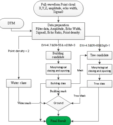
First each pixel is classified using the decision tree shown in Fig. 1 including the threshold values. After the first 2 classes, water and building (candidates) are extracted, mathematical morphology is applied to refine the building results. The pixels not classified are then tested for fulfilling the vegetation criteria. If they are not in vegetation, they are considered to be ground.
Water is first identified, based on the low point density. As mentioned above, water has very low backscatter, and often no detected echo.
Building objects are distinguished from other objects by height (above 3m) and surface roughness. ER is used to distinguish buildings from tree objects. However, with various shapes of building roof and some buildings being covered by high trees, only ER is not sufficient and would include vegetation in the building class. Thus, EW is used to detect only hard surfaces. Buildings are contiguous objects and have typically a minimum size. This is considered by analysing all the pixels classified as buildings so far with mathematical morphology. A closing operation is applied first to fill up all small holes inside the
buildings, and then opening is performed to remove few pixel detections (“noise”) from the building set. This also makes the outlines of buildings smoother.
Figure 1. Decision tree for the classification.
ER, Sigma0 and EW are then used to classify trees. The building mask is applied to classify only pixels not classified before. Also this result is refined with image morphological operations. Finally, all pixels not classified so far are considered ground.
3.4 Echo Width normalisation
An initial assumption was that the thresholds for the decision tree derived for one data set can also be used for the other data set. The rational was that:
Density is a physical measure (points per square meter) and the overall shot density was similar (8 vs. 10 points per square meter).
Height above ground (nDSM) is a measure independent of the measurement device and also independent of the sampling distance.
Echo Ratio is by definition a relative measure and should therefore adapt itself to the data distribution. Sigma0 is the local plane fitting accuracy. For data
sets of similar measurement accuracy (same sensor model used for both areas) and similar neighbourhoods, both number of neighbours and spatial extent, it should deliver comparable values. Echo width obviously depends on the width of the
emitted pulse (same sensor model used for both data sets), but may also depend on the footprint diameter (which was different in the two data sets investigated) or other effects.
Assuming that each data set contains some bright, flat surfaces (orthogonal to the incident Lidar signal), a minimum echo width, EWmin, was chosen based on single echoes (i.e. extended targets) of high amplitude and narrow width. A maximum echo width, EWmax, was chosen based on the assumption that in each data set tree crowns can be found. Those cause large echo width. Thus, strong, first-of-many echoes with a large width were chosen for a maximum echo width. One way to find specific values of EWmin and EWmax is to use quantiles of the distribution of echo width and amplitude. Using quantiles is suggested because of their robust stochastic properties.
The normalized value of EW for the two datasets can then be computed using:
min max
min
EW EW
EW EW NorEW
(2)
It is noted that this can lead to negative normalized EW, which may be left as they are or set to zero. Also values larger than 1 can appear, e.g. for very wide echoes not considered in the normalization due to low amplitude.
A different method to normalize EW value is proposed by (Lin, 2015) which used concept of Fuzzy Small membership.
4. RESULT AND DISCUSSION
4.1 Classification results
The thresholds for the classification were set manually, based on exploratory analysis of the data sets and on expectation of the objects. This was done for both data sets independently.
The main properties of ER, EW, Sigma0, nDSM, and Density values for both Eisenstadt and Vienna are summed up in Table 1. From that properties and combining with empirical selection, the threshold for each parameter was set in the Table 2.
ER [%] EW [ns] Sigma0[m] nDSM [m] Density [pt/m2 ]
Eisenstadt 4.2-100 0-29 0-19 -1.52 – 39 0-72.4 Vienna 2.5-100 .,003-66 0-3474 -1 – 884 0-63
Table 1. The range of ER, EW, Sigma0, nDSM, Density for Eisenstadt and Vienna.
Building Tree Water
ER EW nDSM ER EW Sig.0 Density Eisenstadt >55 <4.7 >3 <60 >4.5 >1 <2 Vienna >55 <9.8 >2 <60 >9.6 >1 <2
Table 2. The threshold values using for decision tree classification of buildings, trees and water body region for
Eisenstadt and Vienna.
The results were evaluated quantitatively and qualitatively. Based on the point density characteristic of water region it produces a good result. All the water bodies in the interested area are classified. However, some small parts of the study area where the laser signal could not reach the ground because of occlusion by high buildings, are misclassified. This could possibly be improved with the overlap of another strip.
While buildings in general can be classified well, very complex roof shapes and walls cause difficulties. It was observed that selecting threshold conservatively the shape of the building is maintained, while its size is reduced slightly.
The tree class includes high trees but also lower vegetation (bushes, etc.), also at heights below 3m. Especially for the latter category EW proofed helpful in distinguishing between vegetation and building edges and also in identifying single trees. For very tall trees, Sigma0 and ER allow reliable detection.
Figure 2. Urban full-waveform classification in Eisenstadt.
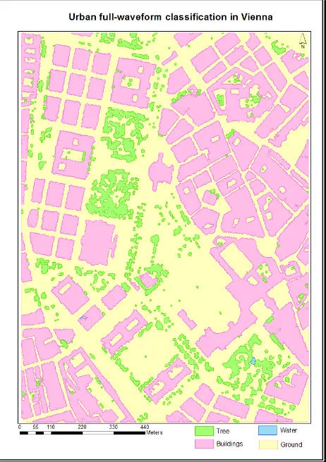
Figure 3. Urban full-waveform classification in Vienna.
The final classification results were then assessed based on Correctness and Completeness (Heipke et al., 1997). Some buildings, trees and water bodies are digitized manually as reference data. Comparing the results of the automated extraction to reference data, an entity classified as an object that also corresponds to an object in the reference is classified as a True Positive (TP). A False Negative (FN) is an entity corresponding to an object in the reference that is classified as background, and a False Positive (FP) is an entity classified as an object that does not correspond to an object in the reference. A True Negative (TN) is an entity belonging to the background both in the classification and in the reference data.
Figure 4. (a) Ground truth data; (b) classified result; (c) accuracy assessment
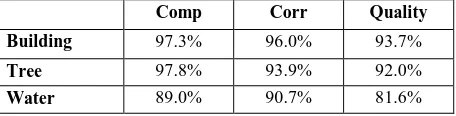
The Completeness and Correction for building, tree, and water class are given in Table 3. It is also illustrated for one building in Figure 4. The two main classes of building and tree feature
Table 3. Accuracy assessments of Building, Tree and Water classes in Eisenstadt region.
4.2 Echo width normalisation
After estimate the threshold values, a comparison of the used thresholds for both regions is carried out to find which parameters keep stable through different dataset and which required to be normalised. As can be seen in the table 2, the threshold of ER, nDSM, Sigma0and Density can be applied for both Eisenstadt and Vienna. In other words, those values can be transferable between different regions. However, the EW threshold is notably different. Thus, the normalization suggested in Sec. 3.4 was applied to evaluate its usability.
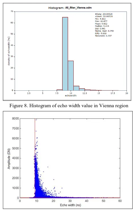
The Figure 5 and Figure 8 show the distribution of EW for the two regions. The ranges of EW are unexpected wide, from found in the data set. Thus, only 5% of all “strong” echoes have a shorter EW than this EWmin. (See Figures 6 and 9). The
maximum EW is chosen as the 99% quantile of EW from the strongest third of the first-of-many echoes with the highest amplitude (Figures 7 and 10). The thresholds for normalizing EW for Eisenstadt and Vienna are summed up in Table 4:
EW
Min Max Mean Std
Eisenstadt 4.4000 9.1000 4.632 0.295 Vienna 8.9480 16.7190 9.538 0.404
Table 4. The EW thresholds for Eisenstadt and Vienna
Applying the normalization, the threshold for normalized EW in Eisenstadt and Vienna are presented in Table 5 While the normalization brings those values closer together (buildings have normalized EW below 6% and 11% respectively, and trees have normalized EW above 3% and 9% respectively), they are not as close together as for the other thresholds (Table 2).
Building Tree
EW EW
Eisenstadt <0.064 >0.027
Vienna <0.106 >0.085
Table 5. Normalized EW thresholds for Eisenstadt and Vienna.
Comp Corr Quality
Building 97.3% 96.9% 94.4%
Tree 93.5% 93.3% 87.6%
Table 6. Accuracy assessments of Building, Tree classes in Eisenstadt region after Echo Width normalisation.
Another way of evaluating the normalization is to apply the thresholds on normalized echo width from one dataset for classifying the other data set. The Eisenstadt values applied to Vienna led to a result of lower quality, but the Vienna thresholds applied to Eisenstadt did produce qualitatively a very similar classification. The completeness and correctness measures are shown in Table 6 . The loss in completeness and correctness does not change for the building class and is below 5% for the tree class.
5. CONCLUSION
This study used full-waveform LiDAR data to classify urban areas, i.e. Eisenstadt and Vienna. Four classes were built: Water bodies, Buildings, Trees and Ground. The computations were executed in OPALS, ArcGIS and FugroViewer. Overall, a high accuracy (>93%) could be achieved.
Full-waveform LiDAR with its additional attributes is an advanced data to classify urban area. The echo width proofed valuable in classifying vegetation and buildings reliably. The other attributes used were Echo Ratio, Sigma0, nDSM, and Density.
Figure 5. Histogram of echo width value in Eisenstadt region
Figure 6. Eisenstadt dataset: Scatterplot of Echo Width versus Amplitude for single echoes. Echoes with more than 1% of the highest Amplitude are placed above the red horizontal line. The vertical line shows the minimum echo width EWmin which is 5% quantile of the single echoes above the Amplitude threshold.
Figure 7. Eisenstadt dataset, Scatterplot of Echo Width versus Amplitude for the first-of-many echoes. The red horizontal line separates the weak (66.6%) from the strong echoes (“highest third”). The vertical line shows the maximum echo width EWmax
which is the EW at the 99% quantile of the strong echoes.
Figure 8. Histogram of echo width value in Vienna region
Figure 9. Vienna dataset: Scatterplot of Echo Width versus Amplitude for single echoes. Echoes with more than 1% of the highest Amplitude are placed above the red horizontal line. The vertical line shows the minimum echo width EWmin which is 5% quantile of the single echoes above the Amplitude threshold.
Figure 10. Vienna dataset: Scatterplot of Echo Width versus Amplitude for the first-of-many echoes. The red horizontal line
separates the weak (66.6%) from the strong echoes (“highest third”). The vertical line shows the maximum echo width EWmax
For the two different study areas the threshold applied for Echo Ratio, Sigma0, and nDSM were the same. Echo Width was shown to depend on the flight mission parameters. The cause was not studied, but the footprint size may have influence. It is noted that using the differential cross section, instead of echo width would not necessarily change this. The differential cross section is obtained by deconvolving (Jutzi and Stilla, 2006; Roncat et al., 2011) the received signal with the emitted pulse shape (more precisely the system waveform).
A simple model for normalizing echo width was suggested. Improvements of this model, e.g., choice of minimum and maximum echo width for normalization, could be investigated, e.g. histogram matching.
ACKNOWLEDGEMENTS
This work is partly founded from the European Community’s Seventh Framework Programme (FP7/2007–2013) under grant agreement No. 606971, the Advanced_SAR project.
The authors would also like to thank VIED (Vietnam International Education Development) and OeAD (Österreichischer Austauschdienst) scholarships for their support in studying period.
REFERENCES
Alexander, C., Tansey, K., Kaduk, J., Holland, D., Tate, N.J., 2010. Backscatter coefficient as an attribute for the classification of full-waveform airborne laser scanning data in urban areas. ISPRS Journal of Photogrammetry and Remote Sensing 65, 423-432.
Ducic, V., Hollaus, M., Ullrich, A., Wagner, W., Melzer, T., 2006. 3D Vegetation mapping and classification using full-waveform laser scanning, in: Forestry., P.o.t.W.o.D.R.S.i. (Ed.), EARSeL/ISPRS, Vienna, Austria, pp. 211–217.
Heipke, C., Mayer, H., Wiedemann, C., 1997. Evaluation of automatic road extraction, IAPRS "3D Recontruction and Modeling of Topographic Objects", Stuttgart, pp. 151-160.
Höfle, B., Mücke, W., Dutter, M., Rutzinger, M., 2009. Detection of building regions using airborne lidar - A new combination of raster and point cloud based GIS methods study area and datasets, International Conference on Applied 395 Geoinformatics. Proceedings of GI-Forum 2009, Salzburg, Austria, pp. 66-75.
Jutzi, B., Stilla, U., 2006. Range determination with waveform recording laser systems using a Wiener Filter. ISPRS Journal of Photogrammetry and Remote Sensing 61, 95-107.
Kraus, K., Pfeifer, N., 1997. A new method for surface reconstruction from laser scanner data, ISPRS Workshop, Haifa, Israel.
Lemmens, M., 2009. Airborne Lidar Sensors. GIM International 2, 16-19.
Lin, Y.-C., 2015. Normalization of Echo Features Derived from Full-Waveform Airborne Laser Scanning Data. Remote Sensing 7, 2731-2751.
Mallet, C., Bretar, F., 2009. Full-waveform topographic lidar: State-of-the-art. ISPRS Journal of Photogrammetry and Remote Sensing 64, 1-16.
Mallet, C., Soergel, U., Bretar, F., 2008. Analysis of Full-waveform LiDAR data for classification of urban areas, The International Archives of the Photogrammetry, Remote Sensing and Spatial Information Sciences, Beijing, pp. 85-92.
Matikainen, L., Hyyppä, J., Ahokas, E., Markelin, L., Kaartinen, H., 2010. Automatic Detection of Buildings and Changes in Buildings for Updating of Maps. Remote Sensing 2, 1217-1248.
Otepka, J., Ghuffar, S., Waldhauser, C., Hochreiter, R., Pfeifer, N., 2013. Georeferenced Point Clouds: A Survey of Features and Point Cloud Management. ISPRS International Journal of Geo-Information 2, 1038--1065.
Pfeifer, N., Mandlburger, G., 2008. Filtering and DTM Generation, in: Shan, J., Toth, C. (Eds.), Topographic Laser Ranging and Scanning: Principles and Processing. CRC Press, pp. 307--333.
Pfeifer, N., Mandlburger, G., Otepka, J., Karel, W., 2014. OPALS – A framework for Airborne Laser Scanning data analysis. Computers, Environment and Urban Systems 45, 125-136.
Roncat, A., Bergauer, G., Pfeifer, N., 2011. B-spline deconvolution for differential target cross-section determination in full-waveform laser scanning data. ISPRS Journal of Photogrammetry and Remote Sensing 66, 418-428.
Rutzinger, M., Höfle, B., Hollaus, M., Pfeifer, N., 2008. Object-Based Point Cloud Analysis of Full-Waveform Airborne Laser Scanning Data for Urban Vegetation Classification. Sensors 8, 4505-4528.
Vetter, M., Hö fle, B., Rutzinger, M., 2009. Water classification using 3D airborne laser scanning point cloud. Österreichische Zeischrift für Vermessung & Geoinformation 97(2), 227-238.
Vosselman, G., Maas, H.-G., 2010. Airborne and terrestrial laser scanning. Whittles Publishing, Dunbeath.