LIDAR DATA RESOLUTION VERSUS HYDRO-MORPHOLOGICAL MODELS FOR
FLOOD RISK ASSESSMENT
A. Avanzi a, E. Frank a, Marika Righetto a, S. Fattorelli a
aBeta Studio srl, 35020 Ponte S. Nicolò (Padova),
Italy. www.betastudio.it, [email protected]
KEY WORDS: LiDAR, topographical resolution, hydro-morphological model
ABSTRACT:
Uncertainties in topographic data have a significant influence on hydro-morphological and hydraulic predictions and therefore on flood risk assessment. In this work, the effects of topographic data resolution on the results of hydro-morphologic and hydraulic simulations are analysed using respectively the morphological bi-dimensional curvilinear model MIKE 21C and mono-bidimensional SOBEK. The studies have been carried out in the Torre river, located in Northern Italy. The evaluations on hydro-morphological and hydraulic risk require accurate spatial information for the area of interest. In order to characterize the river morphology, mainly for large areas, the availability of high resolution topography derived by airborne laser scanner represents an effective tool. Nowadays LiDAR (Light Detection And Ranging) DTM covering large areas are readily available for public authorities, and there is a greater and more widespread interest in the application of such information for the development of automated methods aimed at solving geomorphological and hydrological problems. For the models analysed, high-resolution LiDAR data were used to create the basic topographic information. An additional source for the topography of the Torre river has been provided by river cross-section data. Digital elevation models at different resolution have been created to test the effects of different grid cell sizes on the simulations. The impact of topographic information on hydraulic and morphological model results was evaluated for the area through a comparison of results. Additionally, morphologic variations and position of erosional and depositional zones along the watercourse and variations in flood extent and dynamics have been investigated. The obtained results emphasise the importance of quality of input information for reliable results of hydraulic and sediment transport models. Criteria for selecting the optimal DTM resolution are suggested, based on the quality of available data.
1. INTRODUCTION
Accurate representation of topography and appropriate resolution of data used to perform simulations are of prime importance in hydraulic and morphological modelling. Although, the first point has been studied by many researchers, (Lane & Richards, 1998; Marks & Bates, 2000; Horrit & Bates, 2001; Haile & Rientjes, 2005; Brath et al. 2006; Casa et al., 2005; Wright et al., 2008) the second has been scantily treated. There is often a dilemma in selecting the resolution of Digital Terrain Model (DTM): coarse resolution DTMs usually result in a lower topographical accuracy, but they require a smaller computational effort, while high-resolution ones better represent reality, but they lead to an excessive computational time.
Modern technologies offer nowadays a large number of solutions to obtain and process high quality data and the development in airborne remote sensing data capturing techniques (LiDAR-Light Detection ad Ranging) offers a new support to the use of high-resolution data (Pirotti et al., 2013). Therefore, in practical cases, it is important to evaluate the effects of input data resolution (Pirotti & Tarolli, 2010), especially on modelling simulations.
The aim of this paper is to study the effect of topographic data (LiDAR, cross-section) and spatial model resolution on hydraulic and hydro-morphological variables simulated with the mono/bi-dimensional model SOBEK and the bi-dimensional model MIKE 21C.
This study indicates that different resolutions on topographic data produce important dissimilarities in simulation results, concerning morphological variations (distribution of sediment transport patterns, erosion rates) and flow hydraulics (flow mitigation, propagation time, flood extents).
Comparing model results obtained with different grid dimensions, from higher to lower resolution, important details are lost, mainly as a consequence of averaging and internal interpolations of elevation data, which influences model performance and the reliability of simulation results.
2. DESCRIPTION OF THE MODELS
In this study, the hydro-morphological variables have been simulated with the bi-dimensional model MIKE 21C developed by DHI (DHI, 2005), while flood simulations have been made through the integrated 1D-2D raster based SOBEK flow modelling system developed by WL|Delft Hydraulics.
The modelling of flows within the channel, in both cases, is based on equations of continuity and conservation of momentum (De Saint Venant equations). These equations are solved by implicit difference techniques, with variables defined on a space-staggered computational grid.
In MIKE 21C the hydrodynamic solution is used to evaluate solid transport and the continuity equation of the sediment. The model updates at each time step the curvilinear grid and it represents erosion and deposition processes dynamically, considering a feedback between sediment transport and hydrodynamic conditions.
In SOBEK, to represent 2D flow fields, water is transferred to the adjacent floodplains when bankfull depth is exceeded, and flow is described in the 2D domain in terms of continuity and mass flux equations (Wright et al., 2008).
Both models require topographic information and boundary and initial conditions. Additionally, MIKE 21C requires sediment characteristics of bed (mean diameter, number of fractions, layer thickness and sediment fraction maps), and model coefficients (resistance, helical flow, transverse slope, etc).
2.1 Study Areas
The hydro-morphological simulations have been carried out for the river Torre (A in Fig. 1), while the flood modelling has been performed in an alluvial plain placed on the Adige river right bank. (B in Fig. 1).
Figure 1. Location of the study areas: Reach of the river Torre (A) studied with the MIKE 21C simulations and Adige floodplain (B) studied with the SOBEK model (1. Adige River;
2. pumping station; 3. road embankment; 4. drainage channel)
The river Torre rises in the Italian Dolomites (north-east Italy) and flows for 66 km until it ends at the confluence with the river Isonzo. Its braided riverbed is formed of central islands partially covered with vegetation and extended floodplain areas, often used for agriculture.
The portion of Torre analysed in this work is 12 km long (slope, S = 0.0046 = 0.46%) and it is characterised by peak discharge of 670 m³/s (TR =100 years) for a precipitation of 12 hours (BETA Studio, 2006).
The riverbed is mainly composed of gravel, with a mean grain size (D50) varying between 90 and 10 mm, which dominates the sediment movement. The reach is crossed by several structures (bridges, dams) that influence its hydraulic and morphological behaviour.
Instead the flood modelling study area is an alluvial plain of about 8.3 km² crossed by a road embankment. In case of a bank break or a bank overflowing, water from Adige river would flow across the plain in the south-southeast direction and the road embankment (no. 3 in Fig.1-B) would act as a barrier influencing the flow path.
2.2 Input data of the models
For both study areas, high-resolution LiDAR data with point density varying between 0.3 - 6 point/m², have been used to correctly represent topography.
To model bathymetry within the MIKE 21C, an additional data source model has been provided by field surveys of 15 river cross-sections (numbered from 58 to 43), separated by approximately 900 m, with an average width of 170 m.
DTM derived from cross sections was obtained by joining the principal points (upper-down banks on the right and left sides and bottom) through five 3D-lines drawned according to orthophotos and the Regional Technical Map.
2.2.1 Input data for hydro-morphological simulations: A
curvilinear grid of the riverbed was constructed, considering floodplains and following the streamline directions, stream banks, levees, hydraulic structures, etc.
Five computational grids with different resolution were constructed (Fig. 2).
The main characteristics are listed in Table 1.
Two digital terrain models (2 m x 2 m grid) were generated from the basic topographical information, the first from LiDAR
data (bathymetry „a‟) and the second from cross-sectional data
(bathymetry „b‟). These constituted the input data for the
automatic generation of the curvilinear grid bathymetry in the MIKE 21C model.
Figure 2. Curvilinear grids constructed with different cell dimensions. Grid order is shown according to refinement
Table 1. Characteristics of computed grids. Average cell dimensions in cross-sectional direction (dn), in motion direction
(ds), and number of cells is reported for each grid
Grid number
Average dimensions Number of grid cells dn
(m) ds (m)
dA, area (m²)
Cross-sectional direction
Motion direction Total
1 7 29 205 29 452 13108
2 10 42 426 20 318 6360
3 12 52 659 16 255 4080
4 22 88 1998 9 149 1342
5 49 177 8995 4 74 296
2.2.2 Input data for flood simulations: LiDAR data have
been used to create DTMs with 2.5, 5, 10, 20, 40 and 80 m grid cell size.
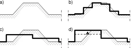
As already seen, the study area is crossed by a road embankment that influences the hydraulic simulation: the smaller cell dimensions can better represent the embankment (Fig. 3b), while the larger grid dimension (20, 40 and 80 m) corresponds to a rougher representation.
With larger grid sizes, height averaging process connected to
data interpolation causes an underestimation of embankment‟s
top (Fig. 3c).
To overcome this problem, new DTMs have been created for each resolution, correcting the elevation of the cells located over the embankment, with new values corresponding to embankment actual height (Fig. 3d).
Figure 3. Cross section schematization of road embankment (a) and grid model representation: b) high resolution DTM, c) low resolution DTM and d) low resolution DTMs modified.
2.3 Boundary conditions
For hydro-morphologic modelling, a flood with TR = 20 years was used as inlet boundary condition (peak discharge 459 m³/s) and a variable water depth calculated according to the hydrograph was set at the outlet section.
A null value of bed level change was assumed both upstream and downstream, in order to avoid numerical instabilities.
a) b)
c) d)
Sediment transport at the inlet was considered to be zero, due to the presence of a dam at the beginning of the reach.
Solid transport has been described exclusively as bedload, due to gravels movement, estimated with the empirical equation of Smart and Jaeggi [10].
Three sediment fractions (15, 30 and 50 mm) were used to describe grain size distribution in the channel, and two homogeneous reaches were defined with different percentages of these fractions.
For flood modelling, two series of hydraulic simulation (each one considering the six grid resolutions) have been performed: the first series uses the DTMs automatically generated from LiDAR points, while the second one uses DTMs modified to simulate the presence of the road embankment. For simulations run with modified DTMs, the 1D flow module is also applied, to represent the drainage channel.
For each simulation, the water level at the end of the drainage channel (upstream the pump station) has been used as a downstream boundary condition, while a triangular shaped inflow hydrograph (TR = 50 years) has been set as an upstream boundary condition.
A constant value of Manning‟s roughness (0.04) has been set for all simulations according to previous analyses (Fattorelli and Frank [11]).
3. RESULTS
The impact of topographic information on hydraulic and morphological model results was evaluated for both areas through a comparison of results obtained for different input data.
Regarding hydrodynamic results, the following comparisons are presented: liquid peak discharges at the outlet of the studied reach, lag time between upstream-downstream peak discharges, maximum water levels in a representative portion of the river reach, and morphologic variations and position of erosional and depositional zones along the watercourse.
For flood simulation, analyses of flooded area dynamics and extent of flood upstream and downstream the road embankment are considered.
In order to analyse the effect of model resolution on the position of erosional and depositional areas along the watercourse for
where A(•) gives the surface classified as above (deposition) and below (erosion) the threshold (± 10 cm) for the hydro-morphological model or the area predicted as inundated by the flood modelling. The indexes Aobs and Asim indicate the
reference and simulated surfaces.
The results obtained with bathymetry „a‟ and grid 1 and the
inundation extent according to the 2.5 m modified DTM are assumed to be the reference values for the hydro-morphological model and for the hydraulic one, respectively, because they presents the best resolution condition.
The value of F indicates if the model parameters are correctly predicted, and may range between F = 1, in case of perfect fit (identical results are obtained) and F = 0, if there is no intersection between simulated and observed areas.
3.1.1 Hydro-morphological model results: Liquid peak
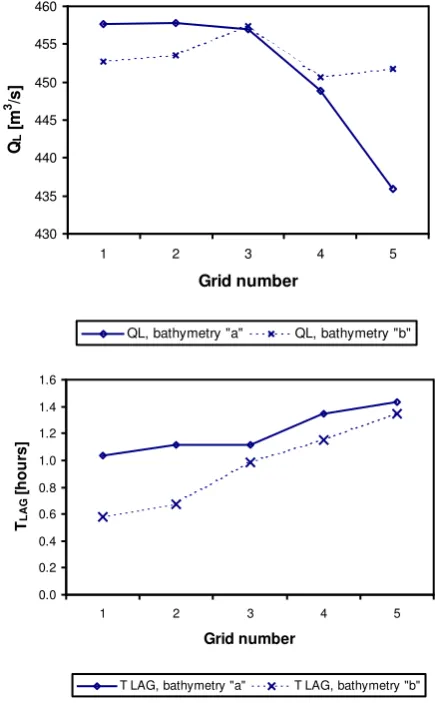
discharges (QL) at the outlet of the reach, calculated with different grid dimensions and the two model bathymetries, are shown in the Fig. 4a.
Note that the peak discharges obtained with LiDAR topographic data, show similar values for the three first grids, and thereafter decrease.
The lag time (Fig. 4b) increases from grid 1 to grid 5. With decreasing grid resolution, there is a smoothing effect of riverbed irregularities, which generates larger cross-sections and lower water depths.
As a consequence, slower flow and higher flood wave mitigation are produced. Considering the cross-sectional data, note that, for the different grids, the QL values are similar, while lag times are lower than the corresponding ones calculated with LiDAR data.
These tendencies may be explained by the raw bathymetry effect, due to the lack of data between cross- sections. This generates a bathymetry with fewer curves (straight channel) and does not describe accurately the morphological features (islands, bars), resulting in a lag time that, for grid 1, is almost half that calculated with bathymetry „a‟.
The same effect due to grid size described above for bathymetry
„a‟ is also observed in this case.
430
QL, bathymetry "a" QL, bathymetry "b"
0.0
T LAG, bathymetry "a" T LAG, bathymetry "b"
Figure 4. Comparison of: (a) liquid peak discharges downstream of reach; (b) lag time for hydrodynamic simulation
with different resolution data (grid and model bathymetry)
An example of simulated maximum water level, with different resolutions of topographical model and grid dimensions, is shown in Fig. 5.
The greater dissimilarity is produced with model bathymetry
„b‟, originating from the traditional topographical survey. In this case, using the largest cell dimension (grid 5) causes uniformity of maximum water levels, which is greater than the smallest cell dimension (grid 1).
This is clear considering that the riverbed is more homogeneous and morphological bed details like central and point bars are lost (Fig. 5).
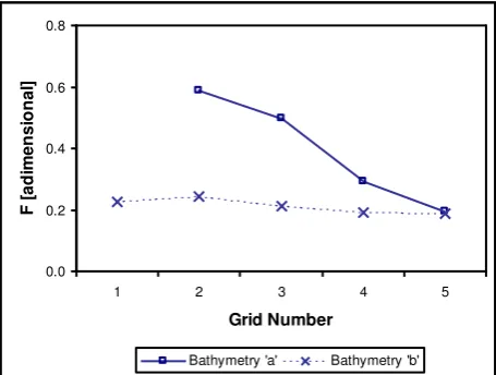
Considering the position of erosional and depositional areas along the watercourse for the Torre river, values of F (Eq. 1)
obtained with bathymetry „a‟ for grids 2-3 (Fig. 6) are close to 0.6, showing good spatial representation of erosional-depositional areas, while with grids 4-5, the F values decrease to 0.29-0.20, indicating that, in those cases, the results are not able to describe the spatial distribution accurately.
Obviously, these results are due to the grid dimension effect, as discussed above.
Figure 5. Comparison of simulated maximum water depth
with different topographical resolutions (bathymetries „a‟-„b‟) and cell sizes (grids 1 to 5)
Figure 6. Comparison of F values, with LiDAR and the cross-section topographic data (bathymetries „a‟-„b‟)
The results obtained with the above statistic can also be observed in Fig. 7, in which the erosional-depositional areas are similar for simulation done with grids 1 and 3 with both bathymetries, but they are highly different when using grid 5 as input. It is also important to highlight the great difference
between grids 1 and 5 on the area spatial distribution obtained with both bathymetries.
The F values obtained with bathymetry „b‟ (around 0.20) indicate that, for all grids, even the one with the highest resolution, the model cannot identify the spatial distribution of erosional-depositional areas with enough precision.
This, of course, is due to the lack of data between two consecutive cross-sections.
Figure 7. Erosional-depositional areas in a portion of the watercourse obtained with grids 1, 3, 5, and bathymetries „a‟-„b‟
3.1.2 Flood modelling results: In simulations run using only
2D module, drainage effect due to channel presence is correctly represented only with high resolution DTMs.
With coarser DTMs (10, 20, 40 and 80 m), the water boards on the plain permanently, since the drainage channel is not detected due to cell dimensions (fig. 8).
DTMs modifications and schematization of the drainage channel through the 1D module, assure better drainage dynamics' simulations for each resolution (Fig. 9).
0.00
0.00 12.00 24.00 36.00 48.00 60.00 72.00 84.00 96.00 108.00
Time (hr)
Figure 8. Inundated Areas Dynamics for different resolution of automatically generated DTMs
0.00 12.00 24.00 36.00 48.00 60.00 72.00 84.00 96.00 108.00
Time (hr)
Figure 9. Inundated areas dynamics for modified DTMs
Considering flood modelling, modification on DTMs slightly influence inundated area upstream the embankment, while downstream areas variation harder reflect road embankment presence and embankment detection (Fig. 10).
Outputs derived from simulations run with 20 m modified DTM are similar to outputs derived from 2.5 and 5 m automatically
Upstream road embankment (A) Downstream road embankment (A) Upstream road embankment (B) Downstream road embankment (B)
Figure 10. Comparison of F values, for different DTM grid size for automatically produced DTM (A) and modified ones (B)
3.1.3 Simulation time: The simulation time using large cells
for hydro-morphological and hydraulic simulations change drastically, according to the grid size.
For the MIKE21C simulations, computational time is 1.5 minutes for grid 5 and increases with grid resolution up to 33 minutes for grid 1.
For flood simulation, simulation takes about 15 minute for the 80 m grid, while the 2.5 m DTM required days of computational time.
This may become critical when dealing with diverse hydrological scenario, corresponding to flood waves of different return time, TR, has to be simulated, resulting in a simulation time of several days.
4. CONCLUSIONS
When a hydraulic or a hydro-morphological model is applied, the availability of topographic data influences the results that can be obtained; the dimensions of the cells should be chosen according to the morphological features present on the study areas.
The analysis carried out in this study, applying the bi-dimensional hydro-morphological model MIKE21C and the mono-bidimensional model SOBEK, indicates that resolution topographic data and cell dimension models produce considerable dissimilarities in simulation results; both on morphological variations (distribution of sediment transport patterns, erosion rates) and hydraulic results (lag time, water depth, flood extent).
Using models based on high-resolution LiDAR data, accurate simulations of hydraulic and hydro-morphological variables were obtained.
A comparison between model results obtained with different grid dimensions highlights important ground feature loss, mainly derived from averaging and internal interpolations of elevation data, which influences model performance and reliability of simulation results.
The analysis on the flood simulations, also, revealed that the use of detailed topographic information itself is not enough to ensure a correct hydraulic representation of surfaces, since this representation depends upon DTM resolution and it is strictly
connected to computational time, that needs to be consistent with study requirement.
This study indicates that optimum choice for grand-scale analysis could be a low resolution DTM processed to represent correctly natural or artificial features (road embankments, minor water streams) that strongly influence flood paths.
Concerning embankments (roads, railways), effectiveness on representation of top height is essential, concerning drainage network, use of coupled 1D-2D models is the key for model reliability.
In case of detailed analysis, instead, it is necessary to choose a digital terrain model with a small cell dimensions; DTMs resolution should be suitable to guarantee a greater reliability of ground feature representation.
For hydro-morphological simulations, raw bathymetric data generated from field surveys (cross-sectional data) produced a smoothing of topography between cross-sections and a consequent loss of morphological details, which does not allow accurate definition of the position of erosional-depositional areas.
Larger grid dimensions reveal as well a gradual loss of detail in the description of topography, and therefore, difficulties in reproducing the characteristics of morphological evolution. Instead, small cells accurately described sediment transport processes or feature that might influence flood dynamics, but they increase the calculation time.
Analysis of the spatial distribution of erosional-depositional areas simulated using LiDAR input data shows that up to 16 cells (grid 3) used in the cross-sectional direction, gives sufficiently accurate results.
This may be explained by considering that, in a braided river, it is essential to have a minimum number of cells on the cross-sectional direction in order to describe each of the existing morphological features (bars, islands, multi-channels, etc.). A lower number of cells (grids 4 and 5) do not describe all these features well enough.
5. REFERENCES
References from Journals:
Brath, A. & Di Baldassarre, G. 2006. Effetti del grado di
dettaglio dell‟informazione topografica nella simulazione
numerica bidimensionale. L’Acqua, 1, pp. 25-30.
Casa, A., Benito, G., Thorndycraft, V.R. & Rico, M. 2005. ground and aerial laser scanning technologies for high-resolution topography of the earth surface. European Journal of Remote Sensing, 46:66-78. doi: 10.5721/EuJRS20134605
Pirotti, F., Tarolli, P., 2010. Suitability of LiDAR point density and derived landform curvature maps for channel network extraction. Hydrological Processes. 24(9), pp. 1187-119. doi: 10.1002/hyp.7582
Lane, S.N. & Richards, K.S. 1998. High resolution, two-dimensional spatial modelling of flow processes in a multi-thread channel. Hydrological Processes, 12, pp. 1279-1298.
Marks, K. & Bates, P. 2000. Integration of high-resolution topographic data with floodplain flow models. Hydrological Processes, 14, pp. 2109-2122.
Wright, N.G., I. Villanueva, P.D. Bates, D.C. Mason, M.D. Wilson, G. Pender, and S. Neelz, A 2008. Case Study of the Use of Remotely-sensed Data for Modelling Flood Inundation on the River Severn, UK,. Journal of Hydraulic Engineering, 134(5).
References from Books:
DHI (Danish Hydraulic Institute). 2005. MIKE 21C, scientific documentation.
References from Other Literature:
Haile, A.T. & Rientjes, T.H.M. 2005. Effects of LiDAR DEM resolution in flood modelling: a model sensitivity study for the
city of Tegucigalpa, Honduras. Workshop “Laser scanning 2005” Enshede, Netherlands, pp. 168-173.
BETA Studio srl. 2006. Progetto preliminare per il ripristino dell'officiosità idraulica del torrente Torre mediante modellazione idraulica dell'asta del torrente torre dalla diga di Crosis, in comune di Tarcento, fino alla confluenza col Fiume Isonzo al fine della messa in sicurezza del territorio. Regione Autonoma Friuli - Venezia Giulia. Protezione Civile della Regione, OPI CD2/430.064.
Smart, G.M. & Jaeggi, M.N.R. 1983. Sediment transport on steep slopes. Mitteilung der Versuchsanstalt für Wasserbau, Hydrologie und Glaziologie der ETH Zurich, 64, pp. 19-76.
Fattorelli, S., Frank, E. 2004. A distributed technique for flood damage assessment using GIS and a 2D hydraulic model. River Basin Management III, WIT Press, Southampton (UK), pp. 433-442.