TOWARDS GUIDED UNDERWATER SURVEY USING LIGHT VISUAL ODOMETRY
M.M. Nawaf∗, P. Drap, J.P. Royer, D. Merad, M. Saccone
Aix-Marseille Universit´e, CNRS, ENSAM, Universit´e De Toulon, LSIS UMR 7296,
Domaine Universitaire de Saint-J´erˆome, Bˆatiment Polytech, Avenue Escadrille Normandie-Niemen, 13397, Marseille, France. [email protected]
Commission II
KEY WORDS:Visual odometry, underwater imaging, computer vision, probabilistic modelling, embedded systems.
ABSTRACT:
A light distributed visual odometry method adapted to embedded hardware platform is proposed. The aim is to guide underwater surveys in real time. We rely on image stream captured using portable stereo rig attached to the embedded system. Taken images are analyzed on the fly to assess image quality in terms of sharpness and lightness, so that immediate actions can be taken accordingly. Images are then transferred over the network to another processing unit to compute the odometry. Relying on a standard ego-motion estimation approach, we speed up points matching between image quadruplets using a low level points matching scheme relying on fast Harris operator and template matching that is invariant to illumination changes. We benefit from having the light source attached to the hardware platform to estimatea priorirough depth belief following light divergence over distance low. The rough depth is used to limit points correspondence search zone as it linearly depends on disparity. A stochastic relative bundle adjustment is applied to minimize re-projection errors. The evaluation of the proposed method demonstrates the gain in terms of computation time w.r.t. other approaches that use more sophisticated feature descriptors. The built system opens promising areas for further development and integration of embedded computer vision techniques.
1. INTRODUCTION
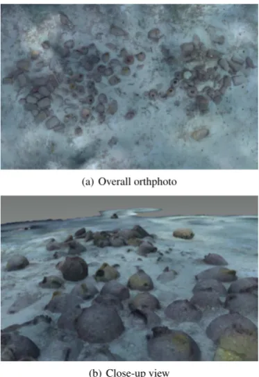
Mobile systems nowadays undergo a growing need for self-localization task to accurately determine its absolute/relative po-sition over time. Despite the existence of very efficient technolo-gies for this purpose that can be used on-ground (indoor/outdoor) and in-air such as Global Positioning System (GPS), optical, ra-dio beacons, etc. However, in the underwater context most of these signals are jammed so that the corresponding techniques cannot be used. On the other side, solutions based on active acoustics such as imaging sonars and Doppler Velocity Logs (DVL) devices remains expensive and requires high technical skills for deployment and operation. Moreover, their size spec-ifications prevents their integration within small mobile systems or even being hand held. The research for an alternative is ongo-ing, notably, the recent advances in embedded systems outcomes relatively small, powerful and cheap devices. This opens inter-esting perspectives to adapt a light visual odometry approach that provides relative path in real-time, which describes our main re-search direction. The developed solution is integrated within un-derwater archaeological site survey task where it plays an impor-tant role to facilitate image acquisition. An example of targeted underwater site is shown in Figure 1.
In underwater survey tasks, mobile underwater vehicles (or divers) navigate over the target site to capture images. The ob-tained images are treated in a later phase to obtain various infor-mation and also to form a realistic 3D model using photogram-metry techniques (Drap, 2012). In such a situation, the main problem is to totally cover the underwater site before ending the mission. Otherwise, we may obtain incomplete 3D models and the mission cost will raise significantly as further exploitation is needed. However, the absence of an overall view of the site
es-∗Corresponding author
(a) Overall orthphoto
(b) Close-up view
Figure 1. Example of a 3D model of an underwater site that is a Phoenician shipwreck recently discovered located near Malta.
quantify visually on the fly. In this work, we propose solutions for the aforementioned problems. Most importantly, we propose to guide the survey based on a visual odometry approach that runs on a distributed embedded system in real-time. The output ego-motion helps to guide the site scanning task by showing ap-proximate scanned areas. Moreover, an overall subjective light-ness indicator is computed for each image to help controlling the lighting and the distance to target which prevents going too dark or overexposed. Similarly, an image sharpness indicator is also computed to avoid having blurred images, and when necessary, to slow down the motion. Overall, we provide a complete hardware and software solution for the problem.
In common approaches of visual odometry, a significant part of the overall processing time is spent on feature points detection, description and matching. In the tested baseline algorithm in-spired from (Kitt et al., 2010), the aforementioned operations rep-resent∼65% of processing time in case of local/relative bundle adjustment (BA) approach, which occupies in return the majority of the time left. Despite their accuracy and successful wide appli-cations, modern features descriptors such as SIFT (Lowe, 2004) and SURF (Bay et al., 2006) rely on differences of Gaussians (DoG) and fast Hessian respectively for feature detection. This is two times slower than the traditional Harris detector (Gauglitz et al., 2011). Further, the sophisticated descriptors that are invariant to scale and rotation, which is not necessary in stereo matching, slow down the computation. And finally, a brute force matching is often used which is also a time consuming. In our proposed method, we rely on low level Harris based detection and template matching procedure. Whereas in traditional stereo matching the search for correspondence is done along the epipolar line within certain fixed range, in our method we proceed first by computing a priorirough depth belief based on image lightness and follow-ing the low of light divergence over distance. This is only valid in a configuration where light sources are fixed to the stereo camera rig, which is the case in our designed system. Our contribution is that we benefit from the rough depth estimation to limit points correspondence search zone since the stereo disparity depends linearly on the distance. The search zone is defined by a prelimi-nary learning phase as will be seen later.
A traditional approach to compute visual odometry based on im-age quadruplets (two distant captures of a stereo imim-age pair) suf-fers from rotation and translation drifts that grows with time (Kitt et al., 2010). The same effect applies to the methods based on local BA (Mouragnon et al., 2009). In contrary, the solutions that are based on using features from the entire image set, such as global BA (Triggs et al., 2000), requires more computational resources which are very limited in our case. Similarly, the simul-taneous localization and mapping (SLAM) approaches (Thrun et al., 2005), which are known to perform good loop closure, are highly computationally intensive especially when complex parti-cle filters are used (Montemerlo and Thrun, 2007). So they can only operate in moderately sized environments if real-time pro-cessing is needed. In our method, we adopt a relative BA method proposed in (Nawaf et al., 2016), which proceed in the same way as local method in optimizing a subset of image frames. How-ever, it differs in the way of selecting the frames subset, as local method uses Euclidean distance and deterministic pose positions to find thek closest frames, the relative method represents the poses in a probabilistic manner, and uses a divergence measure to select such sub set.
The rest of the paper is organized as follows: We survey related works in Section 2. In Section 3 we describe the designed
hard-ware platform that we used to implement our solution. Section 4 presents image quality measurement algorithms. Our proposed visual odometry method is explained in Section 5. The analytical results are verified through simulation experiments presented in Section 6. Finally, in Section 7, we present a summary and con-clusions. Few parts of this work have been presented in (Nawaf et al., 2016).
2. RELATED WORKS
2.1 Feature Points Matching
Common ego-motion estimation methods rely on feature points matching between several poses (Nist´er et al., 2004). The choice of the used approach for matching feature points depends on the context. For instance, features matching between freely taken im-ages (6 degrees of freedom), has to be invariant to scale and ro-tation changes. Scale invariant feature descriptors (SIFT) (Lowe, 2004) and the Speeded Up Robust Features (SURF) (Bay et al., 2006) are well used in this context (Nawaf and Tr´emeau, 2014). In this case, the search for a point’s correspondence is done w.r.t. all points in the destination image.
In certain situations, some constraints can be imposed to facilitate the matching procedure. In particular, limiting the correspon-dence search zone. For instance, in case of pure forward motion, the focus of expansion (FOE) being a single point in the image, the search for the correspondence for a given point is limited to the epipolar line (Yamaguchi et al., 2013). Similarly, in case of sparse stereo matching the correspondence point lies on the same horizontal line in case of rectified stereo or on the epipolar line otherwise. This speeds up the matching procedure first by having less comparisons to perform, and second low-level features can be used (Geiger et al., 2011). According to our knowledge there is no method that proposes an adaptive search range following a rough depth estimation from lightness in underwater imaging.
2.2 Ego-Motion Estimation
Estimating the ego-motion of a mobile system is an old prob-lem in computer vision. Two main categories of methods are de-veloped in parallel, namely; simultaneous localization and map-ping (SLAM) (Davison, 2003), and visual odometry (Nist´er et al., 2004). In the following we highlight the main steps for both approaches as well as hybrid solutions trying to combine their advantages.
SLAM family of methods uses probabilistic model to handle ve-hicle pose, although this kind of methods is developed to handle motion sensors and map landmarks, they work efficiently with visual information solely. In this case, a map of the environment is built and at the same time it is used to deduce the relative pose, which is represented using probabilistic models. Several solu-tions to SLAM involve finding an appropriate representation for the observation model and motion model while preserving effi-cient and consistent computation time. Most methods use ad-ditive Gaussian noise to handle the uncertainty which imposes using extended Kalman Filter (EKF) to solve the SLAM problem (Davison, 2003). In case of using visual features, computation time and used resources grows significantly for large environ-ments. For a complete review for SLAM methods we refer the reader to (Bailey and Durrant-Whyte, 2006).
2004). Based on multiple view geometry fundamentals (Hart-ley and Zisserman, 2003), approximate relative pose can be es-timated, this is followed by a BA procedure to minimize re-projection errors, which yields in improving the estimated struc-ture. Fast and efficient BA approaches are proposed simultane-ously to handle larger number of images (Lourakis and Argyros, 2009). However, in case of long time navigation, the number of images increases dramatically and prevent applying global BA if real time performance is needed. Hence, several local BA ap-proaches have been proposed to handle this problem. In local BA, a sliding window copes with motion and select a fixed num-ber of frames to be considered for BA (Mouragnon et al., 2009). This approach does not suit S-Type motion commonly used in surveys since the lastnframes to the current frame are not nec-essarily the closest. Another local approach is the relative BA proposed in (Sibley et al., 2009). Here, the map is represented as Riemannian manifold based graph with edges representing the potential connections between frames. The method selects the part of the graph where the BA will be applied by forming two regions, an active region that contains the frames with an aver-age re-projection error changes by more than a threshold, and a static region that contains the frames that have common mea-surements with frames in active region. When performing BA, the static region frames are fixed whereas active region frames are optimized. The main problem with this method is that dis-tances between frames are metric, whereas the uncertainty is not considered when computing inter-frames distances.
Recently, a novel relative BA method is proposed by (Nawaf et al., 2016). Particularly, an approximation of the uncertainty for each estimated relative pose is estimated using a machine learn-ing approach manifestlearn-ing on simulated data. Neighborlearn-ing ob-servations used for the semi-global optimization are established based on a probabilistic distance in the estimated trajectory map. This helps to find the frames with potential overlaps with the cur-rent frame while being robust to estimation drifts. We found this method most adapted to our context.
3. HARDWARE PLATFORM
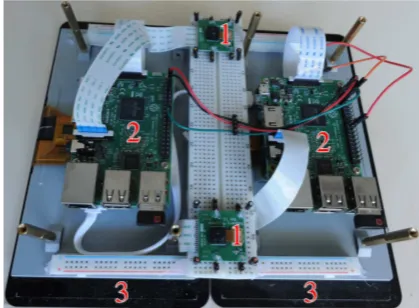
As mentioned earlier, we use an embedded system platform for our implementation. Being increasingly available and cheap, we choose the popular Raspberry Pi c (RPi) as main processing unit of our platform, which is a credit-card size ARM architec-ture based computer running Rasbain c, a Linux variant oper-ating system. Having 1.2 GHz 64-bit quad-core CPU and 1GB of memory allows to run smoothly most of image processing and computer vision techniques. A description of the built system is shown in Figure 2, which is composed of two RPi’s computers each is connected to one camera module to form a stereo pair. The cameras are synchronized using a hardware trigger. Both com-puters are connected to one more powerful computer that can be either within the same enclosure or on-board in our case. Using this configuration, the embedded computers are responsible for image acquisition. The captured stereo images are first partially treated on the fly to provide image quality information as will be details in Section 4. images are then transferred to the main com-puter which handles the ego-motion computation that the system undergoes. For visualization purposes, we use two monitors con-nected to the embedded computers to show live navigation and image quality information (See Figure 3).
Camera stereo pair Embedded computers
Network switch
Storage
Main computer Display
Camera sync signal
Figure 2. System hardware architecture
Figure 3. The hardware platform used for image acquisition and real-time navigation; it is composed mainly of (1) stereo camera
pair, (2) Raspberry Pi c computers and (3) monitors.
4. IMAGE QUALITY ESTIMATION
Since underwater images do not tend to be at best conditions, a failing scenario in computing the ego-motion is expected and has to be considered. Here, we could encounter two cases; First, when having degenerated configuration that causes a failure in estimating the relative motion, this can be due to the bad image quality (blurred, dark or overexposed), the lack of textured areas or large camera displacements. That may raise ill-posed problems at several stages. Second, an imprecise estimation of the relative motion due to poorly distributed feature points or the dominant presence of outliers in the estimation procedure. As the first fail-ure case can be straightly identified by mathematical analysis, the detection of the second case is not trivial. Nevertheless, small er-rors are to be corrected later using the BA procedure.
To estimate image sharpness, we rely on an image gradient mea-sure that detects high frequencies often associated with sharp im-ages, hence, we use a Sobel kernel based filtering which com-putes the gradient with smoothing effect. This removes the effect of dust commonly present in underwater imaging. Given an im-age I, first we compute
G=p
(SK⊤∗I)2+ (KS⊤
∗I)2
(1)
where S= [1 2 1]⊤
K= [−1 0 1]⊤
Next, we consider the sharpness measure to be the mean value of the computed gradient magnitude imageG. The threshold can be easily learned from images by recording the number of matched feature points per image as well as image sharpness indicator. By fixing the minimum number of matched feature points needed to estimate correctly the ego-motion we can compute the minimum sharpness indicator threshold (In our experiments we fix the num-ber of matches to 100 matches, the obtained threshold is 20). It worth to mention that several assumptions used in our work in-cluding this measure does not hold for other above-water imag-ing. The seabed texture guaranties a minimum sharpness even in objects-free scenes, unlike modern above-water scenes.
As mentioned earlier, image lighting conditions play an impor-tant role in computing precise odometry. Similar to image sharp-ness indicator, an image lightsharp-ness indicator can be integrated in the odometry process as well as helping the operator to take proper actions. To estimate lightness indicator, we convert the captured images to CIE-XYZ color space and then to CIE-LAB color space. We consider the lightness indicator as the mean value of theLchannel. The threshold is computed in same way as for the sharpness indicator.
5. VISUAL ODOMETRY
After computing and displaying image quality measures, the im-ages are transfered over the network to a third computer as shown in Figure 2. This computer is responsible for hosting the visual odometry process, which will be explained in this section. We start fist by introducing the used feature matching approach and then we present the ego-motion estimation from image quadru-plets.
5.1 Sparse Stereo Matching
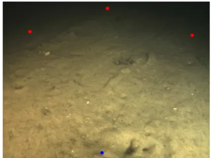
Matching feature points between stereo image pairs is essential to estimate the ego-motion. As the two cameras alignment is not perfect, we start by calibrating the camera pair. Hence, for a given point on the right image we can compute the epipolar line containing the corresponding point in the left image. However, based on the known fixed geometry, the corresponding point po-sition is constrained by a positive disparity. Moreover, given that at deep water the only light source is the one used in our sys-tem, the most far distance that feature points can be detected is limited, see Figure 5 for illustration. This means that there is a minimum disparity value that is greater than zero. Furthermore, when going too close to the scene, parts of the image will become overexposed, similar to the previous point, this imposes a limited maximum disparity. Figure 4 illustrates the aforementioned con-straints by dividing the epipolar line into 4 zones in which one is
an acceptable disparity range. This range can be straightforward identified by learning from a set of captured images (oriented at 30 degrees for better coverage).
Right image Left image
1 2 3 4
Point
Figure 4. Illustration of stereo matching search ranges. (1) Impossible (2) Impossible in deep underwater imaging due to light’s fading at far distances, where features are undetectable (3) Possible disparity (4) The point is very close so it becomes
overexposed and undetectable.
Figure 5. An example of underwater image showing minimum possible disparity (red dots,∼140pixels) and maximum
possible disparity (blue dot,∼430pixels).
In our approach, we propose to constraint the so-called accept-able disparity range further, which corresponds to the range 3 in Figure 4. Given the used lighting system, we can assume a light diffuse reflection model where the light reflects equally in all di-rections. Based on inverse-square law that relates light intensity over distance, image pixels intensities are roughly proportional to their squared disparities. Based on such an assumption we could use feature point’s intensity to constraint the disparity and hence limiting the range of searching for a correspondence. In order to do so, we are based on a dataset of stereo images. For each pair we perform feature points matches. Each point match(xi, yi) and (x′
i, y′i), xbeing the coordinate in the horizontal axis, we compute the squared disparityd2
i = (xi−x′i) 2
. Next, we asso-ciate eachd2
i to the mean lightness value for a window centered at the given point and has a size of2n+ 1computed formL
channel in CIE-LAB color space of the right image as follows:
¯
lxi,yi=
1 4n2+ 4n+ 1
n X
j=−n n X
i=−n
L(xi, yi) (2)
We assign a large valuen = 6to compensate for using Harris operator that promotes local minimum intensity pixels as salient feature points. The computed(¯lxi,yi, d
2
light-ness. A subset of such pairs is plotted in Figure 6.
Figure 6. A subset of matched points squared disparity plotted against average pixel lightness.
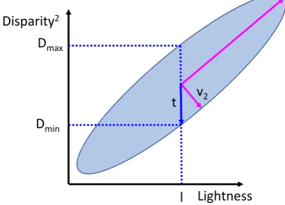
In addition to finding the linear relationship between both vari-ables that allows to give a disparity value for each lightness value, it is also necessary to capture the covariance that represents how rough is our depth approximation. More specifically, given the diagram shown in Figure 7, we aim at defining a tolerancet asso-ciated to each disparity as a function of lightnessl. In our method, we rely on Principal Component Analysis (PCA) technique to ob-tain this information. In details, for a given lightnessli, we first compute the corresponding squared disparityd2
i using a linear
where Dis the training set of disparity,d¯is its mean
Lis the training set of lightness,¯lis its mean
Second, let V2 = (v2,x, v2,y) be the computed eigenvector which correspondences to the smallest eigenvalueλ2. Based on the illustration shown in Figure 7, the tolerancetassociated tod2 i
By considering a normal error distribution of the estimated rough depth, and based on the fact thattis equal to one variance ofD2
, we define the effective disparity range as:
di±γ4
√
t (7)
whereγrepresents the number of standard deviations. It is trivial thatγis a trade-off between computation time and the probabil-ity of having points correspondences within the chosen tolerance
v
2Figure 7. Illustration of disparity tolerancetgiven a lightness valuel.
range. We setγ = 2which means there is95%probability to cover the data.
At this step, we have all the information needed to proceed for the points matching. In which for each feature point in the right im-age, we search for the corresponding point in the left image based on a sliding window over a rectangle whose width is defined by the Equations 3 to 7, and the height is defined empirically to al-low for distortion and stereo misalignment. After testing several distance measures, we found that normalized measures tend to be more robust to underwater imaging. In particular, we use the normalized cross correlation computed as:
R(x, y) = whereWris the sliding window in the right image centered at the query pixel. Ilis the left image. Ris the response that we seek to maximize.
5.2 Ego-Motion Estimation
Since the stereo cameras are already calibrated, their relative po-sition is known in advance. Both cameras have the same intrinsic parameters matrixK. Given left and right frames at timet(we call them previous frames), our visual odometry pipeline consists of four stages:
• Feature points detection and matching for every new stereo pairt+ 1.
• 3D reconstruction of the matched feature points using trian-gulation.
• Relative motion computation using adaptation between the point clouds for the frames attandt+ 1.
• Relative BA procedure is applied to minimize re-projection errors;
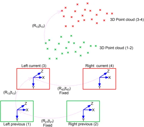
The rigid transformation [R|T] required for expressing the frames at timet+ 1in the reference frame at timetis the rigid transformation required to move the 3D point cloud at timetto the one obtained at timet+ 1. Hence, the problem of calculating the orientation of the cameras at timet+ 1in relation to timet
leads back to the calculation of the transformation used to move from one point cloud to the other. This is possible under our con-figuration, with small rotation. We note here that there is no scale problem between both point clouds which is specific to stereo systems. We consider here the left previous to left current frames
f1 →f3positions to represent the system relative motion, and their relative transformation denoted[R13|T13].
Below, we present the method to compute the transformation for passing from the point cloud calculated at timet+ 1, denotedP, to the one calculated at timet, denotedP′. So we have two sets ofnhomologous pointsP =PiandP′=Pi′where1≤i≤n. We have:
Pi′=R13Pi+T13 (9)
The best transformation the minimizes the errorr, the sum of the squares of the residuals:
r=
n X
i=1
R13Pi+T13−Pi′ 2
(10)
To solve this problem, we use the singular value decomposition (SVD) of the covariance matrix C :
r=
n X
i=1
(Pi−P¯)(Pi′−P¯′) (11)
whereP¯ andP¯′ are the centers of mass of the 3D points sets
P and P′ respectively. Given the SVD of C as: [U, S, V] =
SV D(C), the final transformation is computed as:
R13=V U⊤ (12)
T13=−R13P¯+ ¯P′ (13)
Once the image pairt+ 1is expressed in the reference system of the image pairt, the 3D points can be recalculated using the four observations that we have for each point. A set of verifications are then performed to minimize the pairing errors (verification of the epipolar line, the consistency of the y-parallax, and re-projection residues). Once validated, the approximated camera position at timet+ 1are used as input values for the BA as described earlier.
6. EVALUATION
We implemented our method using OpenCV library and SBA toolbox proposed by (Lourakis and Argyros, 2009). Since our main goal is to reduce the processing time, we tested and com-pared the computation speed of our method comcom-pared to using high level feature descriptors, specifically SIFT and SURF. At the same time, we monitor the precision for each test. The evaluation is done using the same set of images.
In the obtained results, the computation time when using the re-duced matching search range as proposed in this work is∼72%
Figure 8. Image quadruplet, current (left and right) and previous (left and right) frames are used to compute two 3D point clouds. The transformation between the two points clouds is equal to the
relative motion between the two camera positions.
Figure 9. An example of stereo matching using the proposed method
compared1 to the method using the whole search range (range 3 in Figure 4). Concerning SIFT and SURF, the computation time is342%and221%respectively compared to the proposed method. The precision of the obtained odometry is reasonable which is within the limit of 3% for the average translational error and0.02[deg/m]for the average rotational error.
7. CONCLUSIONS AND PERSPECTIVES
In this work, we introduced several improvements to the current traditional visual odometry approach in order to serve in the con-text of underwater surveys. The goal is to be adapted to em-bedded systems known for their lower resources. We resume the developed processing pipeline applied to each captured stereo im-age pair as follows: A sharpness indicator is computed based on quantifying image frequencies, and a lightness indicator is com-puted using CIELAB colour space, both indicators help the op-erator during image acquisition. A sparse feature points detec-tion and improved matching is proposed. The matching is guided with a rough depth estimation using lightness information, this is the factor beyond most of the gain in computation time
com-1
pared to sophisticated feature descriptors combined with brute-force matching.
The evaluation of our system is ongoing. A deep-sea mission is planned in short term in corporation with COMEX2our industrial
partner that provides needed instrumental infrastructure.
Our future perspectives are mainly centered on reducing the over-all system size, for instance, replacing the main computer in our architecture with a third embedded unit, which in turn does not keep evolving. This also allows to reduce the power consumption which increases the navigation time. On the other hand, dealing with visual odometry failure is an important challenge specially in the context of underwater imaging, which is mainly due to bad image quality. The ideas of failing scenarios discussed in this pa-per can be extended to deal with the problem of interruptions in the obtained trajectory.
ACKNOWLEDGEMENTS
This work has been partially supported by both a public grant overseen by the French National Research Agency (ANR) as part of the programContenus num´eriques et interactions (CONTINT) 2013 (reference: ANR-13-CORD-0014), GROPLAN project (Ontology and Photogrammetry; Generalizing Surveys in Un-derwater and Nautical Archaeology)3, and by the French Arma-ments Procurement Agency (DGA), DGA RAPID LORI project (LOcalisation et Reconnaissance d’objets Immerg´es).
REFERENCES
Bailey, T. and Durrant-Whyte, H., 2006. Simultaneous localiza-tion and mapping (slam): Part ii. IEEE Robotics & Automation Magazine13(3), pp. 108–117.
Bay, H., Tuytelaars, T. and Van Gool, L., 2006. Surf: Speeded up robust features. European Conference on Computer Vision pp. 404–417.
Davison, A. J., 2003. Real-time simultaneous localisation and mapping with a single camera. In: Computer Vision, 2003. Proceedings. Ninth IEEE International Conference on, IEEE, pp. 1403–1410.
Drap, P., 2012. Underwater photogrammetry for archaeology. INTECH Open Access Publisher.
Gauglitz, S., H¨ollerer, T. and Turk, M., 2011. Evaluation of in-terest point detectors and feature descriptors for visual tracking. International journal of computer vision94(3), pp. 335–360.
Geiger, A., Ziegler, J. and Stiller, C., 2011. Stereoscan: Dense 3d reconstruction in real-time. In:IEEE Intelligent Vehicles Sympo-sium, pp. 963–968.
Hartley, R. and Zisserman, A., 2003. Multiple view geometry in computer vision. Cambridge university press.
Kitt, B., Geiger, A. and Lategahn, H., 2010. Visual odometry based on stereo image sequences with ransac-based outlier rejec-tion scheme. In:Intelligent Vehicles Symposium (IV), 2010 IEEE, IEEE, pp. 486–492.
Lourakis, M. I. and Argyros, A. A., 2009. Sba: A software pack-age for generic sparse bundle adjustment. ACM Transactions on Mathematical Software36(1), pp. 2.
2
http://www.comex.fr/
3
http://www.groplan.eu
Lowe, D., 2004. Distinctive image features from scale-invariant keypoints. International Journal of Computer Vision 60(2), pp. 91–110.
Montemerlo, M. and Thrun, S., 2007. FastSLAM: A scalable method for the simultaneous localization and mapping problem in robotics. Vol. 27, Springer.
Mouragnon, E., Lhuillier, M., Dhome, M., Dekeyser, F. and Sayd, P., 2009. Generic and real-time structure from motion using local bundle adjustment. Image and Vision Computing27(8), pp. 1178–1193.
Nawaf, M. M. and Tr´emeau, A., 2014. Monocular 3d structure estimation for urban scenes. In:Image Processing (ICIP), 2014 IEEE International Conference on, IEEE, pp. 3763–3767.
Nawaf, M. M., Hijazi, B., Merad, D. and Drap, P., 2016. Guided underwater survey using semi-global visual odometry.15th Inter-national Conference on Computer Applications and Information Technology in the Maritime Industriespp. 288–301.
Nist´er, D., Naroditsky, O. and Bergen, J., 2004. Visual odometry. In:Computer Vision and Pattern Recognition, 2004. CVPR 2004. Proceedings of the 2004 IEEE Computer Society Conference on, Vol. 1, IEEE, pp. I–652.
Sibley, D., Mei, C., Reid, I. and Newman, P., 2009. Adaptive relative bundle adjustment. In: Robotics: science and systems, Vol. 32, p. 33.
Thrun, S., Burgard, W. and Fox, D., 2005.Probabilistic robotics. MIT press.
Triggs, B., McLauchlan, P., Hartley, R. and Fitzgibbon, A., 2000. Bundle adjustment: a modern synthesis. Vision algorithms: the-ory and practicepp. 153–177.