Rank estimation of a generalized
"
xed-e
!
ects
regression model
Jason Abrevaya
*
Graduate School of Business, University of Chicago, 1101 East 58th Street, Chicago, IL 60637, USA
Received 1 July 1997; received in revised form 1 April 1999; accepted 1 April 1999
Abstract
This paper considers estimation of a"xed-e!ects version of thegeneralized regression model of Han (1987, Journal of Econometrics 35, 303}316). The model allows for censoring, places no parametric assumptions on the error disturbances, and allows the "xed e!ects to be correlated with the covariates. We introduce a class of rank estimators that consistently estimate the coe$cients in the generalized "xed-e!ects regression model. Themaximum scoreestimator for the binary choice"xed-e!ects model is part of this class. Like the maximum score estimator, the class of rank estimators converge at less than the Jnrate. Smoothed versions of these estimators, however, converge at rates approaching the Jn rate. In a version of the model that allows for truncated data, a su$cient condition for consistency of the estimators is that the error disturbances have an increasing hazard function. ( 2000 Elsevier Science S.A. All rights reserved.
JEL classixcation: C23; C14
Keywords: Fixed-e!ects models; Generalized regression model; Panel data; Rank es-timators; Maximum score estimator
1. Introduction
Much has been written about the di$culties in consistently estimating the parameters of non-linear "xed-e!ects panel data models. The standard
*Tel.: 001-773-834-0721; fax: 001-773-702-0458.
E-mail address:[email protected] (J. Abrevaya)
"rst-di!erencing trick which eliminates the "xed e!ect from a linear model extends to only certain non-linear models, including the conditional logit model for binary data (Chamberlain, 1980), the Poisson model for count data (Haus-man et al., 1984), and certain parametric models for duration data (Chamber-lain, 1985). Each of these models share an exponential form which allows for cancellation of the"xed e!ect akin to"rst di!erencing in the linear panel model. Semiparametric methods, which do not require any parametric assumptions on the error term, exist for consistent estimation of the binary choice model (Manski, 1987), the linear censored and truncated models (HonoreH, 1992), the selection model (Kyriazidou, 1997), and the dependent-variable transformation model (Abrevaya, 1999).
In this paper, we introduce a class of rank estimators for consistent estimation
of a"xed-e!ects version of thegeneralized regression modelof Han (1987). Like
its cross-sectional counterpart, the model allows for unspeci"ed non-linearity and general forms of censoring. The model allows for correlation between the
"xed e!ects and covariates and does not restrict the "xed e!ects to enter
additively. Themaximum score(MS) estimator for the binary choice"xed-e!ects model (Manski, 1987) is part of the proposed class of estimators. Like the MS estimator, the class of rank estimators converge at less than the Jn rate. Smoothed versions of these estimators, however, converge at rates approaching theJnrate.
In Section 2, we introduce the generalized"xed-e!ects regression model. In Section 3, we propose a class of rank estimators that consistently estimate the coe$cients in the model. Some estimators in the class require i.i.d. error disturbances over time for each cross-sectional unit, whereas other estimators in the class require only a stationarity assumption on the error disturbances. All of the estimators allow for heteroskedasticity across observational units. Smoothed versions of the estimators are also proposed and, applying the results of Horowitz (1992), have convergence rates approaching theJnrate. In Section 4, we discuss estimation when the dependent variable is subject to truncation. For left-truncated data, the assumption that the error disturbances have an increas-ing hazard function (or, equivalently, a log-concave survival function) is su$-cient for consistency. In Section 5, we present Monte Carlo evidence on the small-sample performance of the estimators. Section 6 concludes and discusses some possible extensions.
2. The generalized5xed-e4ects regression model
The generalized regression model of Han (1987) is
yHi"F(x@ ib,ei)
y
i"D(yHi)
where x
i and b areq]1 vectors andei is a i.i.d. error disturbance. The"rst equation describes the &latent' dependent variable yHi, where F: R2PR is strictly increasing in both arguments.Fis an unknown function that allows for unspeci"ed non-linearity in the model. The second equation describes the observed dependent variable y
i, where D: RPY is weakly increasing and non-degenerate. The setYis a subset of the real line that describes the set of
possible dependent variable values. The binary choice model, censored model, and proportional hazards model are examples of (1); see Han (1987) for a discussion. For instance, the binary choice model has F(x@
ib, ei)"
x@ib#e
i,D(yHi)"1 (yHi'0), andY"M0, 1N.
The natural extension of the generalized regression model to a"xed-e!ects setting is cross-sectional unit over time), ande
itis an error disturbance. The number of cross-sectional units,n, is large, whereas the number of time periods is small. For simplicity, we restrict attention to the case of two time periods (t"1, 2). The results extend easily to the case of more time periods and unbalanced panels.1
The"xed e!ectaimay be correlated with the error disturbances, which makes
estimation ofbmore di$cult than in the cross-sectional model. As with other "xed-e!ects estimation techniques, we can only identify the coe$cients of time-varying covariates. Thus,x
itconsists of only time-varying covariates (i.e., those covariates which change with probability greater than zero). Any time-invariant covariates are considered as part of the time-time-invariant"xed-e!ecta
i.
The"rst equation in (2) describes the&latent'dependent variableyH
it, whereFis strictly increasing in its"rst and third arguments. In order to simplify the proof of consistency, we also assume that F is continuous with respect to its third argument. The only di!erence from the model in (1) is thatFhas an additional argument, the "xed e!ect ai. As opposed to most "xed-e!ects models in the econometrics literature, the model in (2) does not restrict the"xed e!ect to be additive. In fact, one could have a vector of "xed e!ects and complicated interactions with the"xed e!ects, e.g.,
yHit"a
1i(x@itb)a2i#a3i#eit, (3) wherea
1i'0 anda2i'0 (to ensure thatFis increasing in its"rst argument).
The model implicitly assumes that D and F do not vary over time. The restriction onDis not substantive, though, since the econometrician can censor the data so that the functionDdoes not vary over time. The time invariance of
Fis crucial for the ranking techniques described below to be applicable. Since F is unspeci"ed in the generalized regression model, the scale and location of b are not identi"ed. As a result, a suitable normalization on b is needed for estimation. To"x the scale ofb, we normalize the parameter vector so that Db1D"1 (i.e., the magnitude of the "rst component of the parameter vector is equal to one).2Corresponding to the normalization onb, de"ne the parameter space of interest,B, as a compact subset ofMb3Rq: Db
1D"1N. We use standard notation to denote"rst di!erences:
*y
i,yi2!yi1, *xi,xi2!xi1, *ei,ei2!ei1.
The"rst di!erence of the independent variables, *x
i, is also aq]1 vector. In a model without a time trend, the constant component can be omitted from the *x
ivector.
When no parametric assumptions are made on the error disturbancese it, there existJn-consistent estimators in the literature for only three special cases of the model in (2):
1. Linear model
F(x@
itb,ai, eit)"x@itb#ai#eit, D(yHit)"yHit.
Ordinary least-squares regression of *y
i on *xi yields a Jn-consistent estimate ofb(including scale and location) if *ei is uncorrelated with*x
i. 2. Censored linear model
F(x@
itb,ai, eit)"x@itb#ai#eit, D(yHit)"yHit)1(yHit'0).
HonoreH (1992) developsJn-consistent estimators forb(including scale and location). The weakest assumption needed for consistency is that the error disturbances are stationary over time for each cross-sectional unit (i.e.,ei1has the same marginal distribution asei2), though this common marginal distri-bution may di!er over cross-sectional units.
3. Transformation model
F(x@itb,ai, eit)"h(x@itb#a
i#eit), D(yHit)"yHit,
wherehis an unknown, strictly increasing function. Abrevaya (1999) develops
Jn-consistent estimators of b (up-to-scale), under the same stationarity assumption described above.
In the"rst two models, bothDandFare known functions, which allows for identi"cation of the location and scale of b. In the last model,F is not fully speci"ed}additivity of the"xed e!ects and error disturbances is assumed, but
his left unknown. IfDand/orFare speci"ed incorrectly in the models above, the estimators forbwill be inconsistent. In this situation, if the data obeys the more #exible model given in (2), the rank estimators of this paper are consistent (up-to-scale). At the very least, these estimators can be used as a speci"cation check when one of the three models above is considered. More importantly, however, these estimators are applicable to the more general model in (2).
The basic idea of rank estimation was"rst utilized by Manski (1987) for the semiparametric binary choice model with"xed e!ects:
F(x@
itb, ai, eit)"x@itb#ai#eit,
D(yH
it)"1(yHit'0).
Themaximum score(MS) estimator ofbmaximizes
Smsn (b)"1
n
n + i/1
M1(*y
i'0))1(*x@ib'0)#1(*yi(0))1(*x@ib(0)N, (4)
based on the idea that it is more likely to seey
i2"1 thanyi1"1 if the index valuex@
i2bis greater than the index valuex@i1b(and vice versa forx@i2b(x@i1b). The MS estimator is consistent under a stationarity assumption on the error disturbances (ei1andei2having the same marginal distribution for each cross-sectional unit). Kim and Pollard (1990) have shown that the cross-cross-sectional MS estimator (Manski, 1975, 1985) converges at the rate ofn~1@3and has a complic-ated limiting distribution. Due to the similarity between the cross-sectional and "xed-e!ects MS estimators, it is quite likely that the proof of Kim and Pollard (1990) can be modi"ed to show that the "xed-e!ects MS estimator also con-verges at raten~1@3. A&smoothed'MS estimator developed by Horowitz (1992), and applied to the binary choice"xed-e!ects model by Kyriazidou (1997) and Charlier et al. (1995), is asymptotically normal with a faster convergence rate. The convergence rate of the smoothed estimator is at leastn~2@5and can be made arbitrarily close ton~1@2, depending on the strength of smoothness assumptions.
3. A class of rank estimators
ranked against each other over time. If x@
i2b'x@i1b, for instance, then the monotonicity ofDandFimplies that it will be more likely to see higher values fory
i2than foryi1(under suitable assumptions on the error disturbances). These comparisons will be valid since each observation corresponding to a given cross-sectional unit has the same "xed e!ect. The estimators will use only within-unit (rather than between-unit) information.
over the parameter spaceB, where the non-degenerate functionH:Y]YPR
is weakly increasing in its "rst argument and weakly decreasing in its second argument:
u
1'u2NH(u1, v)*H(u2,v) ∀v,
v
1'v2NH(u,v1))H(u, v2) ∀u.
The key conditions underlying consistency ofb
nare:
These conditions ensure thatb maximizes the limiting objective function. The rank estimatorb
nis a conditional estimator since only observations with
H(y
i2,yi1)OH(yi1, yi2) can a!ect which parameter vector maximizes (5). When
H(u,v)"1 (u'v), the objective function in (5) is equivalent to the maximum score objective function in (4). Other examples forH(u, v) include:
f H(u,v)"M(u), Mincreasing. f H(u,v)"u/vifYLR`. f H(u,v)"1(u'2v). f H(u,v)"1(u'v))(u!v)2. f H(u,v)"1(u'v))Du!vD.
The objective function in (5) is easy to compute and requires only O(n) calculations. Since the objective function is discontinuous in b, non-gradient search methods (e.g., the Nelder}Mead simplex algorithm) need to be used in order to maximize the objective function.
De,nition. H is separable if &G
1,G2: YPR s.t. H(u,v)"G1(u)#G2(v)∀u,
v3Y.
Separability is related to the assumption on the error disturbances needed for consistency (i.e., for (6) and(7) to hold). A rank estimator with separableH re-quires only stationarity over time of the disturbances for each cross-sectional unit. The maximum score estimator applied to the binary choice model is consistent under stationarity since Y"M0, 1N yields separability. For more general models, though, stationarity is not su$cient for consistency of the maximum score estimator. For such models, rank estimators with separable
Hare consistent under stationarity whereas rank estimators with non-separable
H are consistent under the stronger i.i.d. assumption (i.i.d. over time for each cross-sectional unit, but possibly heteroskedastic across units).
We show that condition (6) holds for general H with i.i.d. errors or for separableHwith stationary errors. By symmetry, condition (7) will also hold. If e1ande2are i.i.d. and*x@b'0, then
E[H(y
2, y1)Dx1,x2,a]"E[H(D)F(x@2b,a, e2),D)F(x@1b,a,e1))Dx1, x2,a]
"E[H(D)F(x@2b,a,e1),D)F(x@1b, a, e2))Dx1, x2, a]
*E[H(D)F(x@1b, a,e1),D)F(x@2b, a, e2))Dx1, x2, a]
"E[H(y
1,y2)Dx1,x2, a].
The i.i.d. assumption gives the second equality. The weak inequality follows sinceFis strictly increasing in its"rst argument. Ife1ande2are stationary and
His separable, then
E[H(y2, y1)Dx1,x2,a]"E[H(D)F(x2@b,a,e2), D)F(x@1b,a, e1))Dx1, x2, a]
"E[G
1(D)F(x@2b,a, e2))
#G
2(D)F(x@1b,a, e1))Dx1, x2, a]
"E[G1(D)F(x@2b,a,e1))
#G2(D)F(x@1b,a, e2))Dx1, x2, a]
*E[G
1(D)F(x@1b,a,e1))
#G
2(D)F(x@2b,a, e2))Dx1, x2, a]
"E[H(y
1,y2)Dx1, x2, a].
In Section 3.1, the regularity conditions for strong consistency are presented. In Section 3.2, a smoothed version of the objective function is introduced to allow for faster rates of convergence. Where possible, the notation from Manski (1987) and Horowitz (1992) is used.
3.1. Consistency
In this section, strong consistency of the class of rank estimators de"ned by (5) is shown. The following assumptions are su$cient to satisfy the conditions of the consistency proof.
The"rst assumption is a standard i.i.d. sampling assumption:
Assumption 1. An i.i.d. sampleM(x
i1, xi2, ai, ei1,ei2): i"1,2,nNis drawn from the population. The observed sample isM(y
i1, xi1, yi2, xi2):i"1,2,nN, where
y
it is generated according to the model in (2). The observed sample has
x
1,x23Rq(q'1) andy1, y23R.
The following two assumptions apply to the error disturbances of the model.
The "rst, a stationarity assumption, is used to show consistency when H is
separable. The second, an i.i.d. assumption, is used to show consistency for any
H.
Assumption E.1. e1ande2are stationary conditional on (x
1,x2, a), with positive density almost everywhere alongR. Denote the common marginal p.d.f. and
c.d.f. byg() Dx1, x2,a) andG()Dx1,x2, a), respectively.
Assumption E.2. e1 and e2 are i.i.d. conditional on (x
1, x2, a), with positive density almost everywhere alongR. Denote the common marginal p.d.f. and
c.d.f. byg() Dx1, x2, a) andG()Dx1,x2, a), respectively.
The functionHmust satisfy some regularity conditions:
Assumption 2. The functionHsatis"es:
(a) u
1'u2NH(u1,v)*H(u2, v) ∀vandv1'v2NH(u, v1))H(u, v2)∀u; (b) E[DH(y
2, y1)!H(y1,y2)D2`g](Rfor someg'0; (c) For anyu3Rand conditional on (x
1, x2, a), eitherH(y1, u) orH(u, y2) is a non-constant random variable.
maximum score objective function, this assumption ensures that both Pr(*y'0) and Pr(*y(0) occur with positive probability.
The following assumption on the covariates is needed for identi"cation ofb:
Assumption 3. (a) The support of the distribution of*xis not contained in any
proper linear subspace ofRq;
(b)b1O0, and for almost every*x8,(*x
2,2,*xq)@, the distribution of*x1 conditional on *x8 has everywhere positive density with respect to Lebesgue measure.
Assumption 3(a) is the usual full-rank condition. Assumption 3(b) is a conti-nuity assumption frequently made in the semiparametric literature.
Finally, we normalize the parameter vector and assume compactness of the parameter space:
Assumption 4. Db1D"1, and bI,(b2,2,bq)@ is contained in a compact subset
BI of Rq~1.
For notational purposes, let bI,(b
2,2,bq)@ denote the last (q!1) compo-nents of any parameter vectorb3Rq. Also, de"ne the parameter space of interest
asB,Mb: Db
1D"1, bI3BI N.
The strong-consistency result is given in the following theorem:
Theorem 1. Let Assumptions 1}4 hold. Letb
nbe a solution to maxb|BS
n(b).If (i)
Assumption E.2 holds or (ii) H is separable and Assumption E.1 holds, then
lim
n?=bn"balmost surely.
The complete proof of Theorem 1 is given in the appendix. The main technicality involves using Assumption 2(c) to strengthen the weak inequalities in conditions (6) and (7) to strict inequalities so thatbis the unique maximizer of the limiting objective function.
3.2. Smoothed estimators
Note that the objective function in (5) is maximized by the same parameter value as
1
n
n + i/1
MH(y
i2, yi1)!H(yi1, yi2)N1(*x@ib'0). (8)
To smooth this objective function, we follow Horowitz (1992) and replace 1(*x@
maximizes the objective function
over the parameter spaceB, where the functionK: RPR and the sequence
Mp
nN=n/1satisfy the following two assumptions:
Assumption 5. (a)Kis a continuous function such thatDK(v)D(M∀vfor some
"niteM; (b) lim
v?~=K(v)"0 and limv?=K(v)"1.
Assumption 6. MpnN=n/1is a positive sequence with lim
n?=pn"0.
Strong consistency is easy to show since the smoothed objective function is a weighted version of the original objective function. Using Assumptions 5 and 6, the proof follows that of Theorem 1 with the additional technicalities handled as in the proof of Lemma 4 of Horowitz (1992). We formally state the strong consistency result in the following theorem:
Theorem 2. Let Assumptions 1}6 hold. Letb
nbe a solution tomaxb|BS
n(b; pn).If(i)
Assumption E.2 holds or (ii) H is separable and Assumption E.1 holds, then
lim
n?=bn"balmost surely.
Extension of the asymptotic normality results of Horowitz (1992) (see also Kyriazidou, 1997; Charlier et al., 1995) is rather straightforward. The key di!erence is that smoothness assumptions on the c.d.f. of the error disturbance (see Assumption 9 of Horowitz, 1992) are replaced by smoothness assumptions on the conditional expectation ofH(y
2,y1)!H(y1,y2) near *x@b"0. Rather than repeating the relevant assumptions and results from Horowitz (1992), we summarize the necessary changes in the appendix.
Horowitz (1992) discusses how to choose the bandwidth for estimation and how to correct the asymptotic bias. The same techniques can be used here as well. Presumably, use of the bootstrap can improve upon asymptotic approxi-mations in"nite samples, as is the case for the smoothed MS estimator of the binary choice model (see Horowitz, 1996).
4. Truncated data
HonoreH (1992), where the data for a cross-sectional unitiare observed only if bothy
i1andyi2are positive (i.e., left truncation at zero).3
We consider a version of the generalized"xed-e!ects regression model in (2) with additive error disturbances:4 an increasing function, there exists some ¸3R such thaty
it'0 if and only if
yH
it'¸. To formalize the truncated sampling, we modify Assumption 1 as follows:
Assumption 1@. An i.i.d. sampleM(x
i1, xi2, ai, ei1,ei2): i"1,2,nNis drawn from the population, conditional on the event y
i1'0 and yi2'0 (where yit is generated according to the model in (10)). The observed sample is M(y
i1, xi1,yi2,xi2): i"1,2,nN, withx1,x23Rq(q'1) andy1, y23R.
Implicit in Assumption 1@ is that the unconditional probability Pr(y
1'0, y2'0) is non-zero.
As before, consistency requires the monotonicity conditions (6) and (7) to hold. Truncation complicates matters since the marginal distributions ofe1and e2are no longer the same after conditioning on observability. Ify
1andy2are observed, it must be the case that e1'¸!F(x@1b, a) and e2'¸!F(x@2b,a). For*x@b'0,e2can take on smaller values thane1, meaning that some sort of shape restriction on the error distribution is needed in order to still&expect'yH2to be larger thanyH1.
Recall thatG() Dx1, x2,a) andg()Dx1,x2, a) are the common marginal c.d.f.
and p.d.f. for the error disturbances. The conditioning arguments will be sup-pressed in what follows. With left-truncated data, a su$cient condition for consistency (in addition to the assumptions from the previous section) is that (1!G) is strictly log-concave (i.e., the logarithm of (1!G) is strictly concave). This condition is equivalent to an increasing hazard functiong/(1!G), since the derivative of log(1!G) is!g/(1!G). The consistency result is formally stated in the following theorem:
3The results of this section can be easily generalized to other forms of truncation. For right-truncated data, a su$cient condition for consistency in Theorem 3 is that the common c.d.f. of the error disturbance is strictly log-concave.
Theorem 3. Let Assumptions 1@, 2}4, and E.2 hold. Let b
n be a solution to
max b|BS
n(b).Assume that G is diwerentiable. If(1!G)is strictly log-concave,then lim
n?=bn"balmost surely.
The proof of Theorem 3 is in the appendix. The basic idea is that for
x@2b'x@1b anda, the log-concavity assumption is su$cient to show that the random variableF(x@2b, a)#e
2stochastically dominates the random variable
F(x@1b, a)#e
1in the "rst-order sense, conditional on both random variables being observed. (When there is no truncation, the stochastic dominance is trivial sincee1ande2have the same marginal distribution andFis strictly increasing in
its"rst argument.)
It is interesting to compare the log-concavity condition of Theorem 3 to the assumption used by HonoreH (1992) for the linear truncated model with
"xed-e!ects.5 HonoreH (1992) assumes log-concavity of the common p.d.f.
g()Dx1,x2, a) of the error disturbances (rather than log-concavity of the
com-mon c.d.f. of the error disturbances). The consistency proof in HonoreH (1992) is based on the symmetry and unimodality of *econditional on (e1#e
2), for which log-concavity of the p.d.f. is needed (see Lemma 1 of HonoreH, 1992). Whether log-concavity of the p.d.f. can be relaxed is unknown, but the unim-odality condition seems essential for identi"cation (see also Powell, 1986, where unimodality is discussed in the cross-sectional version of the estimator). The class of rank estimators, on the other hand, do not require unimodality of*e. The log-concavity assumption of Theorem 3 (i.e., log-concavity of the common survival function) is weaker than the assumption of HonoreH (1992) since
gstrictly log-concaveNGand (1!G) strictly log-concave,
a well-known result in statistics (see Pratt, 1981 or Dharmadhikari and Joag-dev, 1988). The converse is not true. The class of distributions with log-concave
g corresponds to the class of strongly unimodal p.d.f.s, whereas the class of distributions with log-concave (1!G) includes multimodal p.d.f.s. It is straight-forward to construct distributions having multimodal p.d.f.s and log-concave c.d.f.s. The di!erence in log-concavity assumptions is mainly of theoretical interest. As a practical matter, simple simulations by the author have found that the estimators of HonoreH (1992) seem to work"ne when (1!G) is log-concave andgis not.
The results on smoothed estimation from the previous section extend immediately to truncated data once the conditions for consistency are satis"ed.
5. Monte Carlo simulations
In this section, we present some Monte Carlo evidence on the performance of the estimators (both unsmoothed and smoothed versions) for sample sizes of 250 and 1000. The design considered is6
y
t"a(x1t#x2t)#et, t"1, 2, (11) where
x
1t&N(0, 4), x2t"
G
0 if t"1,
1 if t"2, a&U[0, 1], andet&N(0, 1).
Each of the random variables are independent of each other. The second covariate is a time trend. In some sense, the design considered is the simplest possible for the covariates since one component is continuous (needed for identi"cation) and the other has no variation at all. The"xed e!ect is multiplica-tive. (In a model of "rm output, for instance, a could be thought of as an unobserved measure of"rm e$ciency that remains"xed over time.)
Three di!erent rank estimators were used in the simulations, with objective functions:
OBJ1: H(u,v)"1(u'v).
OBJ2: H(u,v)"1(u'v))Du!vD.
OBJ3: H(u,v)"1(u'v))(u!v)2.
OBJ1 is the maximum-score objective function, and OBJ2 and OBJ3 weight observational units by the absolute di!erence in the dependent variable and the squared di!erence in the dependent variable, respectively. For smoothed estima-tion, we report results obtained by using the fourth-order smoothing function used by Horowitz (1992):7
K(v)"
G
0 if v(!5,
0.5#(105/64)[(v/5)!(5/3)(v/5)3
#(7/5)(v/5)5!(3/7)(v/5)7], if !5)v)5,
1 if v'5.
(12)
The results from other smoothing functions were quite similar and, thus, are not reported.
6Other designs were also considered, including designs in which (i) there was dependence between the covariates and the"xed e!ect, and (ii) there was heteroskedasticity of the error disturbance. The basic results were quite similar, so the results from the simplest design are presented.
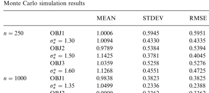
Table 1
Monte Carlo simulation results
MEAN STDEV RMSE MAD
n"250 OBJ1 1.0006 0.5945 0.5951 0.4615
pHn"1.30 1.0094 0.4330 0.4335 0.3312
OBJ2 0.9789 0.5384 0.5394 0.4275
pHn"1.50 1.1425 0.3781 0.4045 0.3144
OBJ3 1.0359 0.5258 0.5276 0.4218
pHn"1.60 1.1268 0.4551 0.4725 0.3481 n"1000 OBJ1 0.9838 0.3823 0.3825 0.3137 pHn"1.35 1.0499 0.2336 0.2388 0.1886
OBJ2 0.9909 0.3362 0.3362 0.2707
pHn"1.45 1.0425 0.2224 0.2263 0.1767
OBJ3 1.0145 0.3397 0.3398 0.2743
pHn"1.60 1.1350 0.2750 0.3060 0.2447
Simulations were performed forn"250 and 1000. In all cases, 500 replica-tions were carried out. Using the normalization from the previous secreplica-tions, the coe$cient of the "rst covariate was held "xed at one. The coe$cient on the second covariate (whose true value is 1) was estimated using a grid search.8 The results are summarized in Table 1, with mean, standard deviation, root-mean-squared error, and mean absolute deviation reported for each estimator.
The "rst row for each estimator corresponds to the unsmoothed estimator.
The second row corresponds to the optimal smoothed estimator (in terms of RMSE), which was determined by doing 500 replications at increments of 0.05 forpn.
The three unsmoothed estimators seem to perform pretty well for both sample sizes. The estimators have very little bias. Not surprisingly, the OBJ1 estimator is somewhat less e$cient (RMSE's 10}15% higher) than the OBJ2 and OBJ3 estimators. The OBJ1 estimator does not use any information about the levels of the dependent variables, only their relative rankings. However, the OBJ1 estimator does have the virtue of being more robust (than OBJ2 and OBJ3) to outliers; see Cavanagh and Sherman (1998) for a discussion. The optimal smoothed OBJ1 and OBJ2 estimators yield substantial e$ciency gains over their unsmoothed counterparts. The smoothed OBJ3 estimator is almost more e$cient than its unsmoothed counterpart, but the bias of the estimator reduces the e$ciency gain (in terms of RMSE) to about 10% for both sample sizes.
Finally, notice that the results in Table 1 are consistent with the slower rates of convergence for the rank estimators. For Jn-consistent estimators, one
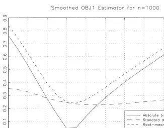
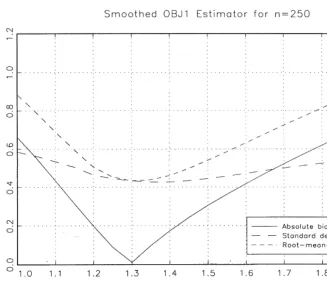
Fig. 1.
would expect the standard deviation or RMSE to halve when the sample size is quadrupled fromn"250 to 1000. The standard deviations for the unsmoothed estimators are about 62}65% lower forn"1000, whereas the standard deviations for the smoothed estimators are about 55}60% lower forn"1000. These num-bers are consistent with the theoretical "nding that the smoothed estimators converge faster than the unsmoothed estimators but slower than theJnrate.
While the smoothed estimators are certainly more attractive from a theoret-ical perspective and perform better than their unsmoothed counterparts when the bandwidth is chosen optimally, Horowitz (1992)"nds that the RMSE of the smoothed estimator is quite sensitive to the bandwidth choice. Our Monte Carlo results also con"rm the sensitivity of the estimates to the bandwidth choice. Forn"250, Fig. 1 graphs the bias (in absolute value), standard devi-ation, and RMSE of the smoothed OBJ1 estimator for di!erent values of the bandwidthp
n. Fig. 2 is the same, except forn"1000. From Table 1, the RMSE of the unsmoothed OBJ1 estimator is 0.5951 for n"250 and 0.3825 for
n"1000. Comparing these values to the RMSE curves in Figs. 1 and 2, the smoothed OBJ1 estimator performs better (in terms of RMSE) for bandwidths between 1.17 and 1.56 forn"250 and for bandwidths between 1.21 and 1.53 for
Fig. 2. Table 2
Bandwidth choice
Region forpnwhere Region relative to
smoothed RMSE( RMSE-minimizing
unsmoothed RMSE bandwidthpHn
n"250 OBJ1 (1.17,1.56) (0.90pHn,1.20pHn) OBJ2 (1.32,1.70) (0.88pHn,1.13pHn) OBJ3 (1.47,1.76) (0.92pHn,1.10pHn) n"1000 OBJ1 (1.21,1.53) (0.90pHn,1.13pHn) OBJ2 (1.35,1.60) (0.93pHn,1.10pHn) OBJ3 (1.52,1.65) (0.95pHn,1.03pHn)
6. Conclusion
This paper has focused on the case of two time periods (t"1, 2). Generalizing the objective function in (5) to more time periods (¹'2) is straightforward:
C
nA
¹ details on the asymptotic theory for¹'2. Computation is still quick since¹is "xed and small.The approach discussed in this paper su!ers many of the same drawbacks as previous papers in the"xed-e!ects estimation literature. First, estimation relies on a strict exogeneity assumption. Dealing with lagged dependent variables in non-linear "xed-e!ects models is a di$cult problem. For instance, HonoreH (1993) has considered moment conditions for estimation of the censored and truncated models with"xed-e!ects and lagged dependent variables, but identi-"cation of the parameter vector is not obtained. More connected to the rank estimators of this paper is HonoreH and Kyriazidou (1997), which considers use of the maximum score estimator for a binary choice"xed-e!ects model with lagged dependent variables. Their approach requires four time periods worth of data as well as additional restrictions on the model (e.g., no time trend between the second and third time periods).
Second, the coe$cients on time-invariant covariates are not identi"ed by the class of estimators. Again, this weakness is shared by other papers in the "xed-e!ects literature. In order to identify these coe$cients, additional exclu-sion restrictions on the"xed e!ects and covariates (e.g., Hausman and Taylor (1981) for the linear model) need to be made. This type of approach is an interesting topic for future research on non-linear"xed-e!ects models.
Further research on the rank estimators described in this paper might focus on issues concerning e$ciency. The choice of H a!ects the e$ciency of the estimators but there is no theory telling the practitioner whichHis`optimala. Cavanagh and Sherman (1998) provide some`rules of thumbafor choosing this function for cross-sectional rank estimators. There may also be e$ciency gains from weighted versions of the rank estimators.
Acknowledgements
Foundation and the University of Chicago GSB research fund are gratefully acknowledged.
Appendix
Proof of Theorem 1. Notice that the objective function S
n(b) has the same
The last term is not a function of b. Consistency will be shown based on the objective functionR
n(b). Denote the limiting objective function by
R
nplaces massn~1at eachzi(adopting the notation of Pakes and Pollard, 1989; Sherman, 1994). MP
nf(), b)!R
0(b): b3BN is a zero-mean empirical process.
We verify the following conditions of Newey and McFadden (1994, Theorem 2.1 (almost-sure version)) needed for strong consistency: (i) R
0(b) uniquely maximized atb; (ii)Bcompact; (iii)R
0(b) continuous; and, (iv)Rn(b) converges uniformly almost surely toR
0(b) (i.e., supb|BDR
n(b)!R0(b)DP!.4. 0). The bulk of the proof involves verifying condition (i), so the other conditions are considered "rst.
Condition (ii) is satis"ed by Assumption 4. Condition (iii) follows directly from the proof of Lemma 5 of Manski (1985). In that proof, continuity relies on the continuity of *x8 from Assumption 3(b), and the existence of the second moment of DH(y
2,y1)!H(y1,y2)D allows use of the dominated convergence theorem. For condition (iv), note that the class of functionsF,Mf(), b):b3BN
is Euclidean for the envelopeDH(y
and Pollard (1989), of whichFis a slight variant). Then, Assumption 2(b) yields condition (iv) by Corollary 9 of Sherman (1994). (Note that weak consistency only requires existence of the second moment; see Corollary 7 of Sherman (1994).
For condition (i), recall from Section 3 that
*x@b'0NE[H(y
2, y1)!H(y1, y2)Dx1,x2, a]*0 (A.1) and
*x@b(0NE[H(y
2, y1)!H(y1, y2)Dx1,x2, a])0. (A.2)
We now show that (A.1) and (A.2) hold with strict inequalities. Without loss of generality, we prove strict inequality for (A.1). Consider any (x
1,x2, a) with *x@b'0. We consider the case of i.i.d. error disturbances and arbitrary H. Extension to stationarity and separability is trivial. By the weak monotonicity of
D,F, andH, we have
E[H(D)F(x@2b, a, e1),D)F(x@1b,a, e2))]
*E[H(D)F(x@1b, a, e1),D)F(x@1b, a,e2))]. (A.3)
Without loss of generality, we know from Assumption 2(c) that H(y
1,u) is a non-constant random variable (conditional on (x
1, x2, a)). (A symmetric argument works for non-constantH(u,y
2).) Thus, for any givene2, there exists someeHs.t. for alle@andeAsatisfyinge@'eH*eA, we have
e@'eH*eANH(D)F(x@2b,a, e@),D)F(x@1b, a, e2))
'H(D)F(x@2b,a,eA),D)F(x@1b, a, e2)).
By monotonicity of Fand continuity in its third argument, there exists some g'0 s.t.
e3(eH!g, eH)NF(x@2b,a, e)'F(x@1b, a, eH).
Combined with the previous inequality, we have
e13(eH!g,eH)NH(D)F(x2@b,a, e1),D)F(x@1b, a, e2))
'H(D)F(x@1b, a,e1),D)F(x@1b, a, e2)).
Since both (A.1) and (A.2) hold with strict inequality for anya, we have
*x@b'0NE[H(y
2, y1)!H(y1, y2)Dx1,x2]'0 (A.4) and
*x@b(0NE[H(y
2, y1)!H(y1, y2)Dx1,x2](0. (A.5) The event M*x@b"0Ncan be ignored since it occurs with zero probability. It follows immediately thatbmaximizes the limiting objective functionR
0(b). To show uniqueness, we need to show that for all other b3B (i.e., bOb),
R
0(b)(R0(b). Given (A.4) and (A.5), it su$ces to show that for anyb3B s.t. bOb, the indicator functions 1(*x@b'0) and 1(*x@b'0) di!er on a region of positive Lebesgue measure. This fact follows immediately from Assumption 3(b); see Manski (1985) or Theorem 2.10 of Newey and McFadden (1994) for details. Thus, condition (i) is satis"ed.
Proof of Theorem 2. Same as Theorem 1, withKhandled as in Horowitz (1992,
Lemma 4).
Proof of Theorem 3. We show that conditions (6) and (7) hold for the truncated
model. Once these conditions are veri"ed, strong consistency follows from the proof of Theorem 1. Veri"cation of (6) and (7) is based on the following lemma:
Lemma 1. Suppose that
yH(z)"F(z)#e,
where F is an increasing function and e is independent of z with diwerentiable
c.d.f. G. IfyH(z)is observed only whenyH(z)'¸andlog(1!G)is strictly concave, then yH(z
1) xrst-order stochastically dominates yH(z2) (in the strong sense) for
z
1'z2.
Proof of Lemma. For ease of exposition, assume that F is di!erentiable with
respect toz. (The argument below can be modi"ed easily to handle a discretized version of di!erentiation.) To show"rst-order stochastic dominance, it su$ces to show that
dPr(yH(z)(cDyH(z)'¸)
dz (0 for anyc'¸.
Note that
Pr(yH(z)(cDyH(z)'¸)"G(c!F(z))!G(¸!F(z))
Di!erentiating with respect tozyields
dPr(yH(z)(cDyH(z)'¸) dz "!
F@(z)(g(c!F(z))!g(¸!F(z))) 1!G(¸!F(z))
!F@(z)(g(¸!F(z))(G(c!F(z))!G(¸!F(z)))
(1!G(¸!F(z)))2 .
We are interested in the sign of this expression. Simplifying and multiplying by (1!G(¸!F(z)))/(1!G(c!F(z))), which doesn't a!ect the sign, yields
!F@(z)
G
g(c!F(z)) 1!G(c!F(z))!g(¸!F(z)) 1!G(¸!F(z))
H
.SinceF@(z) is positive and the hazard function g/(1!G) is strictly increasing (since (1!G) strictly log-concave), this expression is negative. Thus,"rst-order stochastic dominance in the strong sense holds.
By Lemma 1,*x@b'0 implies that the marginal distribution of the random variableyH1"rst-order stochastically dominates the marginal distribution of the random variableyH2. By the monotonicity ofD,F, andH, (6) immediately follows whene1ande2are i.i.d. A symmetric argument for*x@b(0 veri"es condition (7), completing the proof. h
Asymptotic normality of the smoothed estimators: The results of Horowitz (1992)
for smoothed maximum score estimation extend to the smoothed estimators of Section 3.2. A few modi"cations of the assumptions and notation are required. First, x should be replaced by *x to make the results applicable to the "xed-e!ects, rather than cross-sectional, setting.
Then, withz,*x@b, de"ne the following conditional expectation
¸(z, *x8),E[H(y
2, y1)!H(y1, y2)Dz, *x8]. For each positive integeri, de"ne
¸(i)(z, *x8),Li¸(z,*x8)/Lzi
whenever the derivative exists. Assumption 9 of Horowitz (1992) is replaced by:
Assumption. For each integerisuch that 1)i)h, allzin a neighborhood of 0,
almost every *x8, and some M(R, ¸(i)(z, *x8) exists and is a continuous function ofzsatisfyingD¸(i)(z, *x8)D(M.
vectorAand the (q!1)](q!1) matricesDandQby
A,!2a
A h + i/1
M[i!(h!i)!]~1E[¸(i)(0,*x8)p(h~i)(0D*x8)*x8]N,
D,a
DE[E[MH(y2,y1)!H(y1,y2)N2Dz"0,*x8]*x8 *x8 @p(0D*x8)] and
Q,2E[*x8 *x8 @¸(1)(0, *x8)p(0D*x8)],
whenever these quantities exist.9
The main asymptotic results are given by Theorems 2 and 3 of Horowitz (1992). Theorem 2 describes the asymptotic distribution of the smoothed es-timators, and Theorem 3 describes how the quantities in the asymptotic distri-bution can be consistently estimated. In Theorem 3, the only necessary modi"cation is to de"ne
t
i(b, p),(H(yi2, yi1)!H(yi1, yi2))(*x8i/p)K@(*x@ib/p).
References
Abrevaya, J., 1999. Leapfrog estimation of a"xed-e!ects model with unknown transformation of the dependent variable. Journal of Econometrics, forthcoming.
Cavanagh, C., Sherman, R.P., 1998. Rank estimators for monotonic index models. Journal of Econometrics 84, 351}381.
Chamberlain, G., 1980. Analysis of covariance with qualitative data. Review of Economic Studies 47, 225}238.
Chamberlain, G., 1985. Heterogeneity, omitted variable bias, and duration dependence. In: Heck-man, J.J., Singer, B. (Eds.), Longitudinal Analysis of Labor Market Data. Cambridge University Press, New York.
Charlier, E., Melenberg, B., van Soest, A.H.O., 1995. A smoothed maximum score estimator for the binary choice panel data model with an application to labour force participation. Statistica Neerlandica 49, 324}342.
Dharmadhikari, S., Joag-dev, K., 1988. Unimodality, Convexity, and Applications. Academic Press, Boston.
Han, A.K., 1987. Non-parametric analysis of a generalized regression model: the maximum rank correlation estimator. Journal of Econometrics 35, 303}316.
Hausman, J.A., Hall, B., Griliches, Z., 1984. Economic models for count data with an application to the patents-R&D relationship. Econometrica 52, 909}938.
Hausman, J.A., Taylor, W.E., 1981. Panel data and unobservable individual e!ects. Econometrica 49, 1377}1398.
Heckman, J.J., HonoreH, B.E., 1990. The empirical content of the Roy model. Econometrica 58, 1121}1149.
HonoreH, B.E., 1992. Trimmed LAD and least squares estimation of truncated and censored regression models with"xed e!ects. Econometrica 60, 533}565.
HonoreH, B.E., 1993. Orthogonality conditions for Tobit models with "xed e!ects and lagged dependent variables. Journal of Econometrics 59, 35}61.
HonoreH, B.E., Kyriazidou, E., 1997. Panel data discrete choice models with lagged dependent variables. Mimeo.
Horowitz, J.L., 1992. A smoothed maximum score estimator for the binary response model. Econometrica 60, 505}531.
Horowitz, J.L., 1996. Bootstrap critical values for tests based on the smoothed maximum score estimator. Mimeo.
Kim, J., Pollard, D., 1990. Cube root asymptotics. Annals of Statistics 18, 191}219.
Kyriazidou, E., 1997. Estimation of a panel data sample selection model. Econometrica 65, 1335}1364.
Manski, C.F., 1975. Maximum score estimation of the stochastic utility model of choice. Journal of Econometrics 3, 205}228.
Manski, C.F., 1985. Semiparametric analysis of discrete response: asymptotic properties of the maximum score estimator. Journal of Econometrics 27, 313}333.
Manski, C.F., 1987. Semiparametric analysis of random e!ects linear models from binary panel data. Econometrica 55, 357}362.
Newey, W.K., McFadden, D., 1994. Large sample estimation and hypothesis testing. In: Engle, R.F., McFadden, D.L. (Eds.), Handbook of Econometrics, Vol. IV. Elsevier Science, Amsterdam. Pakes, A., Pollard, D., 1989. Simulation and the asymptotics of optimization estimators.
Econo-metrica 57, 1027}1057.
Powell, J.L., 1986. Symmetrically trimmed least squares estimation for Tobit models. Econometrica 54, 1435}1460.
Pratt, J.W., 1981. Concavity of the log likelihood. Journal of the American Statistical Association 76, 103}106.