*Corresponding author. Tel.: 001-206-685-8082; fax: 001-206-685-7477. E-mail address:[email protected] (T.S. Eicher)
q
An earlier version of this paper was presented at the SCE/IFAC Conference, held in Cambridge, UK, June 29}July 1, 1998. The comments of three anonymous referees are gratefully acknowledged. Eicher gratefully acknowledges support from the von Humboldt foundation.
25 (2001) 85}113
Transitional dynamics in a two-sector
non-scale growth model
qTheo S. Eicher
*
, Stephen J. Turnovsky
Department of Economics, University of Washington, Box 353330, Seattle WA 98195, USA Accepted 9 November 1999
Abstract
This paper shows how, under plausible conditions, the transitional dynamics in a two-sector R&D-based non-scale growth model are represented by a two-dimensional stable saddlepath, thus enriching the transitional adjustment paths relative to that of the standard two-sector endogenous growth model. The transition speed itself is variable both through time and across sectors. Capital and knowledge grow at very di!erent rates, consistent with the empirical evidence. Numerical simulations are used to characterize the transition paths in response to a range of speci"c shocks. In some cases, capital or knowledge may overshoot their respective long-run responses, during the transitional dynamics. ( 2001 Elsevier Science B.V. All rights reserved.
Keywords: Transitional dynamics; Non-scale growth
1. Introduction
Transitional dynamics are at the heart of the recent convergence debate. If, and at what rate, countries converge to their respective equilibrium growth paths is intimately tied to the transition behavior of the key determinants of
1Non-scalerefers to the characteristic that variations in the size or scale of the economy do not permanently alter its long-run equilibriumgrowth rate. For example, R&D-based growth models that follow Romer (1990) arescalemodels since they imply that an increase in the level of resources devoted to R&D should increase the growth rate proportionately; see Jones (1995b).
2Mulligan and Sala-i-Martin (1993) established a slightly weaker condition for balanced growth for a Lucas type endogenous growth model.
economic growth: capital accumulation, technological change, and the growth of e!ective labor. The existing literature on convergence addresses this issue using models, such as the one-sector neoclassical model or the two-sector AK endogenous growth model, in which the transitional adjustment locus is one dimensional. In such models, all variables converge at the same constant rate, a consequence of which is that authors emphasize only capital accumulation and its constant speed of convergence during the transition. Only to avoid estimates of excessively high capital shares did Mankiw et al. (1992) introduce human capital to the analysis.
But to assume that the transition of all factors occurs at identical and constant rates is an excessively restrictive assumption. It is more realistic and general to allow factors to converge at di!erential speeds throughout the transition. There is, in fact, robust evidence by Dowrick and Nguyen (1989) and Bernard and Jones (1996b) that suggests that the characteristics of technology during transition are distinctly di!erent from those of capital accumulation.
In this paper we examine the transitional dynamics of a two-sector non-scale growth model that incorporates the endogenous accumulation of technology and capital, in an economy with exogenous population growth.1The model has several appealing features. As in Mankiw et al. (1992) equilibrium growth rates are independent of the size (scale) of the economy, and hence our model also predicts conditional convergence. Indeed, the invariance of long-run growth rates with respect to scale is supported by empirical evidence for OECD countries (Jones, 1995a) as well as for the United States (Backus et al., 1992). Also, in contrast to the previous one-sector neoclassical and two-sector endo-genous growth models, the transitional dynamics are now generated by more
#exible paths, thus permitting technology to evolve independently of the time paths of capital and labor, again consistent with the empirical evidence cited above.
3Arnold (1998) obtains a third-order dynamic system by treating the value of consumption expenditure as numeraire, thereby holding the shadow value of wealth constant.
4Strictly speaking, this remark refers to the speed of convergence of the linearized system, which is what most studies consider. The true speed of adjustment of a"rst-order non-linear system will in general be time-varying.
5Benhabib and Perli (1994) show how an extension of the Lucas model to include endogenous labor and labor externalities may generate a third-order dynamic system having two stable roots. This will give rise to a two-dimenional stable adjustment path, that is associated with multiple equilibria, in contrast to the non-scale model in which the equilibrium is generally found to be unique.
e!ects. From this standpoint, non-scale growth equilibria should be viewed as being the norm, rather than the exception, and consequently it is even more important that their dynamic properties be characterized.
Examples of non-scale models have been introduced by Jones (1995a), Seger-strom (1998) and Young (1998). Eicher and Turnovsky (1999) have provided a comprehensive framework to allow for a general characterization of non-scale balanced growth equilibria in two-sector models. But no comprehensive analy-sis of the transitional dynamics of this class of models exists. This constitutes a severe limitation to our understanding of the steady-state behavior, since without an understanding of the underlying dynamics, it is by no means clear that the economy will reach its equilibrium. Furthermore, even if the system is stable, the relevance of the steady-state balanced growth path depends upon how rapidly key variables converge to their respective steady states along the transitional path. Jones (1995b) sketched the transitional dynamics of a
simpli-"ed two-sector non-scale economy. To reduce the dimensionality of his system, however, he assumed that sectoral labor allocation and investment rates are exogenous constant. A complete analysis requires that these variables be endo-genously determined as part of the dynamic equilibrium.3This is done in our investigation below, where we"nd dramatic (qualitative) variation of the sec-toral allocation of labor during the transition, this being a re#ection of the complexity of the transitional path, itself.
6The empirical evidence on the constancy of convergence rates is mixed. Barro and Sala-i-Martin (1995), who abstract from technological change, can reject constancy for Japan, but not for the US or Europe. Nevertheless, all reported rates of convergence (0.4}3%, 0.4}6%, and 0.7}3.4% for Japan, the US, and Europe respectively) are similar in the range that our non-scale model generates.
7This contrasts with overshooting familiar from the one-dimensional transitional path, which always occurs only on impact with the arrival of new information and is therefore not generated by the system's internal dynamics.
The existence of two-dimensional transition paths introduces important new characteristics to the transition. First, in contrast to the Lucas, AK, or one-sector neoclassical models, the transition no longer occurs at a constant speed. Instead, two-dimensional manifolds imply that the convergence speeds will vary through time and across variables, often dramatically so, hereby introducing important#exibility to the transitional dynamics. Furthermore, the character-istics of the respective transition paths di!er for all endogenous variables. Indeed, one of the key"ndings is that capital and knowledge will grow at very di!erent rates throughout the transition. The implication for empirical research is then that the dynamic properties of two-sector non-scale models may thus address the concerns of Bernard and Jones (1996a,b), since our analysis pro-duces neither common transition paths and rates of convergence, nor common stationary growth rates for all variables.6
To obtain a qualitative impression about the transition, we calibrate the two-sector non-scale model. For completeness, we report three adjustment speeds. First, we plot the time pro"les of capital, technology, and output, in order to highlight di!erences in their transition paths and in their speeds and direction of adjustment. Our calibration results document the wide range of transitional adjustment paths that may result. We show that a necessary condition for monotonic transitions is that the steady-state levels of both variables change in the same direction (i.e., both capital and knowledge increase or decrease). But even if both variables converge monotonically, this does not imply that theirspeedsof adjustment are either constant or identical. Especially interesting are non-monotonic paths that involve &overshooting', in that vari-ables along their transition pathsexceedtheir new long-run equilibrium value. For example, a shock may induce a transition during the initial stages of which the economy decumulates more than the necessary amount of some quantity. The excessive decumulation subsequently requires an accumulation of that quantity during the"nal stages of transition.7
8We use the term`social stocksato refer to the amalgam of private stocks and those representing possible social spillovers. This allows us to specify decreasing, constant, or increasing returns to scale without having to worry about issues pertaining to market structure. As in Mulligan and Sala-i-Martin (1993), the elasticities derived from (1b) refer to the sum of private and social elasticities. positive shock. That is not necessarily the case here. We will present an example where a positive productivity shock in the technology sector leads to a mono-tonic adjustment in both capital and technology, whereas a subsequent reversal of that shock may be associated with highly non-monotonic behavior.
The rest of the paper is organized as follows. Section 2 presents a two-sector model of economic growth. The two sectors we consider are output and a knowledge-producing sector, also referred to as technology and R&D. We begin by deriving the equilibrium conditions and brie#y characterizing the balanced growth path. Section 3 lays out the model's formal dynamic structure. Because a complete formal analysis of the fourth-order system is virtually intractable, our analysis relies on numerical calibration methods, the results of which are presented in Section 4. In that section we "rst identify a plausible benchmark set of parameter values. We then proceed to examine the dynamic adjustment of the economy to various kinds of shocks and structural changes, such as variations in the sectoral productivity parameters, returns to scale, preference parameters, as well as population growth.
2. A two-sector non-scale economy
We begin by outlining the structure of a two-sector non-scale model that features exogenous population growth and endogenously capital and techno-logy. The properties of this base model have been discussed extensively in Eicher and Turnovsky (1999) and so our discussion can be brief, focusing only on those aspects that are most relevant to the dynamics.
We focus on a centrally planned economy and use social production func-tions, in which externalities are internalized. The population,N, is assumed to grow at the steady rateNQ /N"n. The economy produces"nal output,>, and
new technology,A, utilizing the social stocks of technology, labor, and physical capital,K, according to the Cobb}Douglas production functions:8
>"a
FApA[hN]pNKpK, 0(pi(1, i"A,N,K, (1a)
AQ"a
JAgA[(1!h)N]gN!dAA, 0(gi(1, i"A,N, (1b)
wherea
F,aJ represent exogenous technological shift factors to the production functions andhis the fraction of labor employed in the"nal good sector,p
i,gi are the productive elasticities, and d
9This technology is somewhat more general than Jones (1995), who speci"es pA"p N" 1!p
K,p. Eicher and Turnovsky (1999) discuss the balanced-growth characteristics of a general two-sector technology, in which capital enters the production function of new knowledge. The Romer model corresponds to the casep
A"pN"1!pK,gN"gA"1.
10Eicher and Turnovsky (1999) abstract from physical depreciation. We introduce it here, since it is quite important for the purposes of numerical calibration and simulation. The structure along the lines (1b)}(1d) was originally investigated within a traditional Ramsey framework by Shell (1967). technology.9Physical capital accumulates residually, after aggregate consump-tion,C, and depreciation needs,d
KK, have been met
KQ ">!C!d
KK. (1c)
The planner's problem is to maximize the intertemporal utility of the repre-sentative agent:
where C/N denotes per capita consumption, subject to the production and accumulation constraints, (1a)}(1c), and the usual initial conditions. His decision variables are: (i) the rate of per capita consumption,C; (ii) the sectoral allocation of labor,h; (iii) the rates of accumulation of physical capital and technology. The optimality and transversality conditions to this central planning problem can be summarized as follows: physical capital and knowledge. These conditions are standard and have been discussed in Eicher and Turnovsky (1999).10
2.1. Balanced growth equilibrium
facts (Romer, 1989), we assume that the output/capital ratio,>/K, is constant.
A key feature of the non-scale model is that the equilibrium percentage growth rates of technology and capital,AK andKK respectively, are determined entirely by production conditions. Taking the di!erentials of the production functions (1a) and (1b), and solving, we obtain:
AK" gN(1!pK)n
and thus the per capita growth rate of output (capital) is
>K !n"[(1!gA)(pA#pN#pK!1)#pA(gA#gN!1)]n
(1!g
A)(1!pK)
. (3c)
It is evident from (3a) and (3b) that the magnitude of the relative sectoral growth rates depend upon the assumed production elasticities in conjunction with the population growth rate. Eq. (3c) implies that countries converge to identical output per capita growth rates if either their production technologies are identical, or their production functions exhibit constant returns to scale. If production technologies di!er across countries, growth rates exhibit conditional convergence. Jones (1995a) speci"es output to be constant returns to scale in physical capital and knowledge-adjusted labor,AN. The striking feature of the equilibrium growth rate in the Jones model is that per capita consumption, per capita output and capital, and technology all grow at a common rate deter-mined by: (i) the growth rate of labor, and (ii) the elasticities of labor and knowledge in the knowledge-producing sector alone. Any characteristic of the
11Under constant returns to scale these scale-adjusted quantities are just regular per capita quantities.
to scale in both sectors. In particular, scale models of growth attain non-zero growth in the absence of population growth by imposing constant returns to scale in the accumulated factors, K and A. Thus AK or Lucas}Romer type growth models require the knife-edge assumption that g
A"1, and
p
AFinally, the possibly di#pK"1. !erential equilibrium growth rates of physical capital and knowledge are re#ected in the growth rates of their respective shadow values,l,k, which, using the optimality conditions (2), can be shown to grow in accordance with
l(!k("(b
A!bK)n. (3d)
3. Dynamics of a two-sector model
To derive the dynamics about the balanced growth path we de"ne the following stationary variables: y,>/NbK;k,K/NbK;c,C/NbK;a,A/NbA; j,J/NbK;q,l/kN(bA~bK). For convenience, we shall refer toy, k, c, andaas
scale-adjustedquantities.11This allows us to rewrite scale-adjusted output and
technology as
y"a
FhpNapAkpK, (4a)
j"a
J(1!h)gNagA. (4b)
The optimality conditions then enable the dynamics to be expressed in terms of these scale-adjusted variables, as follows. First, the labor allocation condition (2b) can be expressed in the form
a
FqpNhpN~1apAkpK"aJgN(1!h)gN~1agA
enabling us to solve for the fraction of labor allocated to output:
h"h(q,a,k);Lh/Lq'0,Lh/Lk'0, sgn(Lh/La)"sgn(p
The shadow values of capital and technology, determined by (2c) and (2d), can
Taking the time derivative of (2a) and combining with (6a), the growth rate of aggregate consumption is given by
CQ
C"
1
c[pKaFhpNapAkpK~1!((1!c)n#dK#o)]. (6c)
Using these"rst-order conditions the dynamic system can be expressed in terms of the rede"ned stationary variables by
kQ"k
C
hpNawhere his determined by (5). To the extent that we are interested in the per capita growth rates of capital and knowledge, they are given by KQ /K"
kQ/k#(bK!1)n;AQ/A"a5/a#(bA!1)n.
together with the two production functions (4a) and (4b), and the labor alloca-tion condialloca-tion (5). These seven equaalloca-tions determine the steady-state equilibrium in the following sequential manner. First, (8d) determines the output}capital ratio, so that the long-run net return to capital equals the rate of return on consumption. Notice that the elasticity c raises or lowers the long-run out-put}capital ratio depending upon whether b
Kj1. If the production function Jhas constant returns to scale,y8/kI is independent of the production elasticities,
g
N,gA, of the knowledge-producing sector. Likewise, (8b) yields the gross equilibrium growth rate of knowledge, jI/a8"JI/AI, in terms of the returns to scale, b
A, and the rates of population growth and depreciation. Having obtained the output}capital ratio, (8a) determines the consumption}capital ratio consistent with the growth rate of capital necessary to equip the growing labor force and replace depreciation. Giveny8/kI andjI/a8, (8c) implies the sectoral allocation of labor,hI, at which the rates of return to investing in the two sectors are equalized.
GivenhI andjI/a8, the production function for knowledge determines the stock of knowledge,a8, while the production function for output then yields the stock of capital, kI. Finally, having derived hI,a8,kI, the labor allocation condi-tion determines the long-run equilibrium relative shadow value of the two assets,q8.
Linearizing around the steady state denoted bykI,a8,q8,c8, the dynamics may be approximated by the following fourth-order system:
12The characteristic equation for the linearized system (4) is of the form:k4#n
1k3#n2k2# n3k#n
4"0, whereniare functions of the elements ofaijof the matrix in (4). The determinantal
condition (i) impliesn4'0, while the dynamic e$ciency condition (ii) impliesn1(0. By Descartes rule of signs, necessary and su$cient conditions for the characteristic equation to have just two positive roots is that eithern2(0 orn3'0. Conditions (ii) and (iii) noted above are examples of conditions that ensuren2(0 and other more general, but more complicated conditions can also be found. In addition, conditions that su$ce to ensuren3'0 can also be obtained.
a
It is readily shown that the determinant of this matrix is proportional to (g
A!1)(pK!1). Imposing the conditionpK(1,gA(1 implies that the deter-minant is positive which means that it has either 0, 2, or 4 positive roots. The dynamic e$ciency condition, (i)LF/LK,p
K(y8/kI)'bKn, rules out the"rst case.
Unfortunately, due to the complexity of the system, we cannot"nd as general a condition to rule out the case of 4 unstable roots. However, the conditions (ii)
c51, (iii)p
k41/(1#c) are two simple and plausible restrictions that su$ce to eliminate the third case of explosive growth. These conditions are met by our simulations and indeed, in all of the many simulations carried out over a wide range of parameter sets, 2 positive roots were always obtained.12Thus since the system features two state variables,kanda, and two jump variablesc, andq, we are con"dent that equilibrium is characterized by a unique stable saddlepath.
3.1. Characterization of transitional dynamics
Henceforth, we assume that the stability properties are ensured so that we can denote the two stable roots byk1,k2, withk2(k
1(0. The key variables of
interest are physical capital, and technology. The generic form of the stable solution for these variables is given by
k(t)!kI"B
1ek1t#B2ek2t, (10a)
a(t)!a8"B
1l21ek1t#B2l22ek2t, (10b)
where B1,B2 are constants and the vector (1,l2i,l3i,l4i), i"1, 2 (where the prime denotes vector transpose) is the normalized eigenvector associated with the stable eigenvalue,k
i. The constants,B1,B2, appearing in solution (10) are
obtained from initial conditions, and depend upon the speci"c shocks. Thus suppose that the economy starts out with given initial stocks of capital and knowledge, k
In studying the dynamics, we are interested in characterizing the slope along the transitional path in a!kspace. In general, this is given by
da
and is time varying. Note that since 0'k
1'k2, astPRthis converges to the
new steady state along the direction (da/dk)
t?="l21, for all shocks. The initial
direction of motion is obtained by settingt"0 in (12) and depends upon the source of the shock.
It is convenient to express the dynamics of the state variables in phase-space form:
By construction, the trace of the matrix in (13)"k
1#k2(0 and the
determi-nant"k
13Note that the representation of the transitional dynamics ink}aspace takes full account of the feedbacks arising from the jump variables,qandc; these are incorporated in the two eigenvalues.
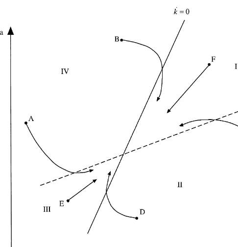
Fig. 1. Two-dimensional transition paths in two-sector non-scale models.
in (10) and (13) are in terms of the scale adjusted quantities, from which the growth rates of per capita capital and knowledge can be derived.13
Eqs. (10a) and (10b) highlight the fact that with the transition path inkand abeing governed by two stable eigenvalues, the speeds of adjustment for capital and knowledge are neither constant nor equal over time. In addition, with output being determined by capital and technology, the transition of output is also not constant over time, but a simple composite of the transition character-istics ofaandkas determined in (13).
14In a converging economy this measure is positive. A negative value implies divergence. Because of the nonlinear stable adjustment path it is possible forx(t) to overshoot its long-run equilibrium,x8, during the transition. If that occurs, then at the point of overshooting, the speed of convergence will become in"nite (positively or negatively, depending upon the direction of motion). Examples of this are provided in Figs. 3 and 4.
marginal physical product of capital, and therefore output, although the in-crease in employment is o!setting. For plausible values ofp
K, the former e!ect dominates requiring an increase ina for equilibrium in the output market to prevail; thus the upward-slopingkQ"0 locus. Moreover, for plausible values, the e!ect through the productivity of capital prevails, in which case the kQ"0 implies the steeper locus, as in our simulations.
Various transition paths are illustrated, indicating the distinct possibilities of overshooting. If we start in region I or III, both capital and technology converge monotonically, which implies that the transition path for output is also mono-tonic. Note that this does not imply that the speeds of adjustment are either constant or identical for capital and technology, Hence the speed of transition of output also varies over time. If we start from points A or C (B or D) it is clear that technology (capital) overshoots its long-run equilibrium level during transition. This leads to strong variations in the rates of growth of technology (capital) during the transition, featuring both above and below long-run growth rates during the adjustment. The asymmetry of the transitional paths to positive and negative shocks occurs if the positive shock occurs when the economy starts from a point in Region I, relative to the new equilibrium, while the reverse negative shock starts if the new equilibrium is in Region relative to the original equilibrium. Examples of this are provided in Figs. 5 and 6.
As noted at the outset, a key issue concerns the speed of convergence; see Barro and Sala-i-Martin (1992) and Ortigueira and Santos (1997). In previous growth models, in which all variables moved in proportion to one another, the associated unique stable eigenvalue su$ced to characterize the transition. With two stable roots 0'k
1'k2, say, the speeds of adjustment change over time,
although asymptotically all scale-adjusted variables converge to their respective equilibrium at the rate of the slower growing eigenvalue,!k
1. In particular,
since scale-adjusted output is determined by capital and technology and the proportion of labor allocated to manufacturing during the transition, its conver-gence speed is also not constant over time, but is a composite of the others.
In general, we de"ne the speed of convergence at timet, of a variablexsay, as
/
x(t),!
A
x5(t)!x85
x(t)!x8
B
(14)15We have conducted extensive sensitivity analysis and found that our results reported below are remarkably robust to changes in the underlying parameters.
constant or follows a steady growth path and the stable manifold is one dimensional, this measure equals the magnitude of the unique stable eigenvalue (see Ortigueira and Santos, 1997). But we are primarily interested in the convergence speeds ofper capitaquantities, in particular, per capita output and technology,>/NandA/N, which in steady-state equilibrium grow at the rates
(b
K!1)n, and (bA!1)n. As usual in endogenous growth models this implies that per capita variables arenon-stationary unless both sectors exhibit overall constant returns to scale. Applying the measure (14) to either per capita variable, we"nd
/
Y@N(t)"!
y5(t)
y(t)!y8!(bK!1)n"/y(t)!(bK!1)n, (15a)
/
A@N(t)"!
a5(t)
a(t)!a8!(bA!1)n"/a(t)!(bA!1)n. (15b)
This has the same time pro"le as does scale-adjusted output, except that its speed of convergence has to be adjusted by the growth rate of per capita output. Asymptotically, /
Y@N(t) converges to its steady-state growth path at the rate
!k
1!(bK!1)n. Thus, per capita output,>/N, will converge slower, or faster than does scale-adjusted output, y, depending upon whether the equilibrium balanced growth rate of per capita output is positive or negative. This in turn depends upon returns to scale. Moreover, although scale-adjusted capital and knowledge both converge asymptotically at the same rate, !k
1, their
corresponding per-capita quantities, K/N,A/N, converge to their respective nonstationary growing equilibrium paths at the di!erential rates
!k
1!(bK!1)n,!k1!(bA!1)n, respectively.
4. Numerical analysis of transitional paths
Table 1
Benchmark parameters
Production parameters aF"1,pN"0.6,pK"0.4,pA"0.3,aJ"1,gN"0.5,gA"0.6 Preference parameters o"0.04;c"1
Depreciation and population parameters d
K"0.05,dA"0.01,n"0.015
Table 2
Benchmark equilibrium values
(>/
Y
N) (A/Y
N) (>I/K) (CI/>) hI /IY@N /IA@N
0.009 0.003 0.285 0.740 0.941 0.0196 0.0256
16See, for example, Prescott (1986), Lucas (1988), Ortigueira and Santos (1997), and Jones (1995b).
17The empirical literature on research functions is sparse, especially if one requires separate elasticities for labor and technology. Adams (1990) and Caballero and Ja!ee (1993) are examples of thorough empirical investigations that are ultimately unsuccessful in reporting separate elasticities for labor and technology. Kortum (1993) derives values of about 0.2 by extrapolating results from aggregate patent data. Jones and Williams (1995) obtain estimates between 0.5 and 0.75, these however, are a function of their assumed rate of growth and the assumed share of technology in research.
4.1. Benchmark economy
Table 1 shows that the values we employ for our fundamental parameters are essentially identical to those used in previous calibration exercises.16The"nal goods sector exhibits constant returns to scale in capital and labor, but increas-ing returns to scale with the inclusion of knowledge. The technology sector is subject to mildly increasing returns to scale in labor and knowledge.17 These assumptions are made so as to obtain a plausible equilibrium per capita output growth rate. Several parameters, such as the rate of time preference and labor growth rate, have a time dimension. In this case the chosen parameters are in annual rates so that the time unit in the simulations represents one year.
We group the resulting endogenous variables into three categories. The
balanced per capita growth ratesof capital (output), and technology;key
equilib-rium ratios, including the output}capital ratio, the share of consumption in
output, and the share of labor employed in the output sector; theconvergence
speedsof per capita capital (output) and technology. All turn out to be
18Given that the elasticities of labor and capital in output are commonly assumed to be around 0.6 and 0.3, respectively, higher per capita growth rates would require greater technology spillovers in production or greater returns to scale in technology. The evidence does not seem to provide su$cient support for either. Alternatively, the long-run growth rate of output may be raised by introducing capital into the production of knowledge. However, the intersectoral allocation of capital (along with labor) complicates the dynamics further, without adding insight.
19Non-scale growth alone is not su$cient to generate realistic speeds of convergence. The one-sector non-scale model can be conveniently parameterized by settingpA"0,gx"0,x"A,
N,K. Its rate of convergence can also be shown to be excessively high, at about 10% p.a. for the benchmark parameter set.
Given the larger increasing returns in the"nal good sector, the growth rate of capital and output of exceeds that of technology, with per capita output growing at nearly 1%, and per capita knowledge at 0.3%.18The capital}output ratio is approximately 3.5, while around 74% of output is devoted to consumption. Approximately 94% of the work force is employed in the output sector, with the balance of 6% employed in producing knowledge. Most importantly, the larger of the two stable eigenvalues, k1, implies that per capita output converges asymptotically at an annual rate of nearly 2%, consistent with the empirical evidence.19The slower per capita growth of knowledge implies that per capita knowledge converges at a faster rate of nearly 2.6%.
We turn now to the numerical analysis of the transitional paths. We seek to provide examples of the non-constant and di!erential rates of convergence of capital and technology, and of the two}dimensional saddlepath. Speci"cally, we provide examples highlighting how such paths allow the economy to overshoot its long-run equilibrium during the transition, an aspect that has not been documented in previous growth models. In addition, the calibration exercise provides examples of the distinct shapes of the transition paths that the model incorporates (as seen in Fig. 1). The best way to highlight these characteristics is to examine the response of the economy to productivity shocks in both the"nal good and knowledge-producing sector and contrast each transition with the e!ects on the economy that would result from a change in the returns to scale.
4.2. Productivity shocks
The long-run e!ects of exogenous changes in the productivity of the "nal output sector and the knowledge-producing sector, as described by changes in the exogenous productivity parametersaF,aJ, are summarized in Table 3, while Figs. 2}6 illustrate the corresponding transitional dynamic adjustments.
This table highlights the non-scale character of the model. None of the key economic variables reported in the table are a!ected by changes in the produc-tivity parameters,a
Table 3
Productivity shocks
(>/
Y
N) (A/Y
N) (>I/K) (CI/>) hI /IY@N /IA@N
aF"2 0.009 0.003 0.285 0.740 0.941 0.0196 0.0256
a
F"2,c"1.5 0.009 0.003 0.296 0.750 0.943 0.0178 0.0238
a
F"2,o"0.10 0.009 0.003 0.435 0.830 0.958 0.0212 0.0271
a
F"2,n"0.025 0.015 0.015 0.325 0.723 0.921 0.0236 0.0336
aJ"2 0.009 0.003 0.285 0.740 0.941 0.0196 0.0256
aJ"0.5 0.009 0.003 0.285 0.740 0.941 0.0196 0.0256
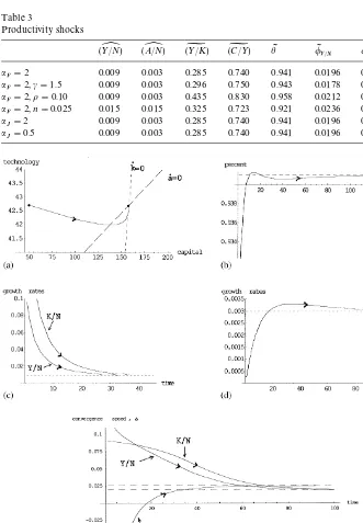
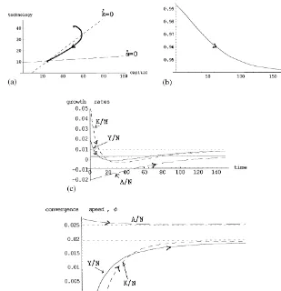
Fig. 3. (a) Scale adjusted capital and technology whileaFincreases from 1 to 2 andcfrom 1 to 1.5. (b) Percentage of labor force in manufacturing whileaFincreases from 1 to 2 andcfrom 1 to 1.5. (c) Time pro"le of per capita growth rates of capital and output, technology. (d) Per capita convergence speeds of capital and output. (e) Per capita convergence speeds of technology.
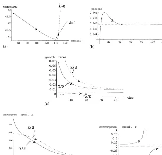
Fig. 4. (a) Scale-adjusted capital and technology whileaFincreases from 1 to 2 andnfrom 0.015 to 0.025. (b) Percentage of labor force in manufacturing whileaFincreases from 1 to 2 andnfrom 0.015 to 0.025. (c) Time pro"le of per capita growth rates of capital and output, technology. (d) Per capita convergence speeds of capital and output. (e) Per capita convergence speeds of technology.
4.2.1. Productivity increase inxnal goods sector
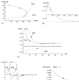
Fig. 5. (a) Scale-adjusted capital and technology whilea
Jincreases from 1 to 2. (b) Percentage of labor force in manufacturing whileaJincreases from 1 to 2. (c) Time pro"le of per capita growth rates of capital and output, technology. (d) Per capita convergence speeds of capital, output and technology.
output production. The transition paths turn out to be remarkably diverse across these changes in parameters, thus highlighting an additional, crucial di!erence between steady states and transitions in the non-scale model.
The dynamic adjustment to a simple increase in the productivity in the"nal sector (a
F"1 toaF"2) is illustrated in Figs. 2a}e. The only long-run e!ect of
Fig. 6. (a) Scale-adjusted capital and technology whileaJdecreases from 1 to 0.5. (b) Percentage of labor force in manufacturing whileaJdecreases from 1 to 0.5. (c) Time pro"le of per capita growth rates of capital and output, technology. (d) Per capita convergence speeds of capital, output and technology.
20The constancy of a across steady states is a consequence of the assumption that the production function of knowledge is independent of capital.
the long-run scale-adjusted stock of knowledge, a8, remain unchanged.20 The transition path in Fig. 2a is thus an example of the path described by the transition from (A) in Fig. 1.
sector, including labor. There is however, a second contemporaneous e!ect. The long-run increase in the stock of capital, with knowledge unchanged lowers its long-run shadow value,q, and given the forward-looking behavior of the model, the short-run value ofqdeclines as well. This reduces the relative productivity of labor in"nal output production, thereby having an o!setting e!ect on employ-ment and attracting it away from that sector. For our chosen set of parameter values this negative e!ect on h dominates, so that initially, and seemingly paradoxically, an increase in productivity in the "nal output sector actually leads to an initial decline in employment in that sector, see Fig. 2b.
The phase diagram, Fig. 2a, shows that initially, the increase in productivity of the output sector attracts resources to that sector, and away from the know-ledge-producing sector. The scale-adjusted capital stock begins to accumulate
and is accompanied by areductionin the scale-adjusted knowledge due to the fact that its per capita rate of accumulation is insu$cient to cover the deprecia-tion rate and populadeprecia-tion growth rate (Fig. 2d). Fig. 2c shows that per capita output and capital growth rates rise dramatically to about 10% during the early stages, after which they fall rapidly toward their long-run steady state of just under 1%. Within 10 periods the growth rate of capital is reduced to around 4%, while that of output is just 2%. Output growth thus adjusts faster than capital growth. Technology growth has a very di!erent pattern. After its initial decline, technology growth overshoots its long-run growth rate. This is because the rapid increase in capital together with the reduction in knowledge during the early stages eventually raises the relative return on investing in knowledge su$ciently, relative to the return on capital.
The nonlinear transitional path for labor allocation mirrors the adjustment paths in capital and knowledge. We have already noted the initial decline in labor employed in"nal output. The initial accumulation of capital attracts more labor to the"nal output sector. In addition, under the assumptionp
A(gA, the initial decline in knowledge further serves to drive labor from the knowledge-producing sector to the"nal output sector. Both these in#uences therefore serve to reverse the initial migration of labor from the "nal output sector and so
hinitially increases rapidly, as illustrated in Fig. 2b. Over time, as the growth rate of capital declines and the decline of knowledge is reversed, this migration of labor toward"nal output is reversed andhbegins to decline again. In the"nal phases, as the magnitude of the overshooting of knowledge declines, the impact of the higher capital stock on labor prevails and during the latter phases
e!ects on the convergence speed. However, the transition is nonlinear across variables and over time. For this reason we report the time pro"le of the convergence speeds. In the case where only the productivity in the"nal sector increases, output remains above its asymptotic speed for a signi"cant period of time, while technology, while"rst diverging, recovers much faster.
Figs. 3 and 4 illustrate the transitional dynamics in cases where the productiv-ity increase in a
F is accompanied by (i) an increase in the intertemporal elasticity of substitution,cfrom 1 to 1.5, an (ii) an increase in the population growth rate from 1.5 to 2.5%, respectively. In the"rst case, most aspects of the transition are broadly similar to those illustrated in Fig. 2, in which c was unchanged. There is, however, one di!erence. The higher rate of return to consumption, and the resulting increase in steady-state consumption, leads to less expansion in the long-run capital stock and prevents the stock of knowledge from being restored to its original level. Accordingly, during the transition,a(t), actually overshoots its new steady-state equilibrium. This occurs after approx-imately 15 years. At that timea(t)"a8, and the corresponding speed of conver-gence of technology,a(t), at that instant as given by (14) becomes in"nite; see Eq. (14). Immediately after passing through that point, while still declining,a(t) is diverging at an in"nite rate, though ultimately this is reversed, and eventually it converges at its asymptotic rate of 2.38%. But it is this overshooting that accounts for the singularity observed in Fig. 1e.
The case where the increase in productivity is accompanied by an increase in the population growth rate gives a distinctly di!erent transition pattern, and is an example for transition path (B) in Fig. 1b. In contrast to Figs. 2 and 3 where the stock of knowledge overshoots during the transition, it now declines mono-tonically, while the stock of capital now overshoots its long-run response. Capital is being accumulated during the early and middle stages of transition and then decumulated during the latter stages of the transition. As in Figs. 2a and 3a, the productivity shock to the "nal output sector induces an initial reduction in investment in knowledge and increase in investment in capital. As kincreases andadeclines, the productivity of knowledge rises, but now by an insu$cient amount to o!set the higher population growth rate, so thata de-clines monotonically. Likewise, the accumulation of capital reduces the produc-tivity of capital such that given the higher population growth rate, it eventually declines as well. The overshooting of capital is associated with an in"nite speed of convergence at that point, for the same reason as just given for knowledge. Moreover, the overshooting of capital leads to overshooting of output, which because of the more rapid adjustment of output, occurs at an earlier stage during the transition (5 y rather than 11).
4.2.2. Productivity increase in knowledge sector
The second group of experiments consists of various parametric changes associated with changes in the productivity of the knowledge sector,a
a
J"2. These shocks are instructive because the transition paths highlight the
fundamental novel characteristics of the non-scale model. First we"nd that the transition paths are quite distinct from those obtained when only the productiv-ity of the "nal output sector is changed. This group of simulations provides a particularly instructive example of the signi"cance of two stable roots and the importance of two-dimensional transition paths; namely the asymmetry with respect to speci"c directional changes of the productivity parameter.
The long-run e!ects of an increase in the productivity of the knowledge-producing sector are summarized in rows 5 and 6 of Table 3, with the corre-sponding transitional dynamics being illustrated in Figs. 5 and 6. As for the corresponding shock in the output sector, the equilibrium quantities remain unchanged from the benchmark case. The transition, however, is markedly di!erent from the previous case. Analogous to the productivity shock in the output sector which increased the steady-state stock of capital, we now"nd that the productivity shock in the knowledge sector raises the equilibrium stock of knowledge,a8. This causes an initial decline in the fraction of labor devoted to
"nal output production, as seen in Fig. 5b. However, now we"nd an additional e!ect. Since the production function for output (4a) implies that an increase in a8 raises the productivity of physical capital, capital must increase as well, in order for its average product, y8/kI, to remain constant. Thus in contrast to a productivity shock in the output sector, an increase in the productivity of the knowledge-producing sector leads to long run increases in the stocks ofboth
knowledge and physical capital, although the increase is heavily biased toward the latter.
The transitional adjustments are markedly di!erent from our previous cases.
An increase in the productivity in the knowledge sector causes monotonic
adjustment, in contrast to the overshooting during the transition in the case when the productivity in the"nal goods sector rises. The adjustment path when only the productivity of the research sector is increased (Fig. 5a) serves as an example for a transition from point E in Fig. 1b.
The increase in productivity in the technology sector attracts resources to that sector, so that the growth rate of knowledge initially rises above 8% for knowledge, 4% for output, and 1.5% for capital (Fig. 5c). The growth rate of capital also rises initially, but at a slower rate than technology, due to the fact that the expansion in capital occurs as a result of the higher stock of knowledge, which takes time to accumulate.
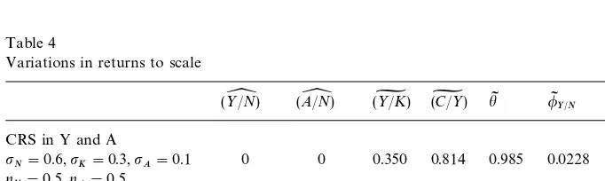
Table 4
Variations in returns to scale
(>/
Y
N) (A/Y
N) (>I/K) (CI/>) hI /IY@N /IA@N CRS in Y and A
pN"0.6,pK"0.3,pA"0.1 0 0 0.350 0.814 0.985 0.0228 0.0228
gN"0.5,gA"0.5 DRS in Y and A
p
N"0.55,pK"0.25,pA"0.1 !0.0024 !0.0027 0.411 0.847 0.986 0.0231 0.0234
g
N"0.45,gA"0.45
labor to back to output production, while the latter has the opposite e!ect. The former e!ect dominates and the fraction of labor employed in output gradually increases back to its initial equilibrium level.
To illustrate how di!erent the speed of adjustment might appear, depending upon initial conditions and the direction of the shock, we also report a change in the productivity of research for the case wherea
Jdeclines from 1 to 0.5. Initially, one might think that halving the productivity would simply imply a reverse transition to doubling it, as in Fig. 5. But that is not the case Capital overshoots its long-run level (Fig. 6a) and the transition path is now similar to (B) in Fig. 1b. The growth rate of capital rises signi"cantly above its long-run growth rate, and together with output returns nonmonotonically to the equilibrium.
4.3. Changes in returns to scale
The responses to the productivity shocks summarized in Table 3 share several important characteristics. First, key aspects of the equilibria do not depend upon the shift terms,a
F,aJ. This is a manifestation of the non-scale aspects of the models, since, these parameters can be viewed as embodying scale e!ects. The other interesting feature was the examples of drastically di!erent transition paths that involve overshooting on the part of both technology and capital during alternative transition paths. In addition, the asymptotic speed of adjust-ment is robust to (plausible) changes in the underlying parameters.
Thus far, returns to scale have been held"xed at 1.3 in the case of output, and 1.1 for the production of knowledge. Table 4 considers variations in the degrees of returns to scale. In the"rst case we subject both sectors to mildly diminishing returns to scale, while the second example assumes constant returns to scale in both sectors.
and then to decreasing returns to scale raises the share of labor in the "nal output sector. As the positive spillover of technology in the production of"nal output is reduced it is less attractive to allocate labor to research. On the other hand, the speeds of convergence are hardly a!ected.
5. Conclusions
In this paper we have examined the transitional dynamics of a new class of growth model, one characterized by non-scale e!ects. Two issues have moti-vated our interest in this class of model. First, despite the existence of empirical evidence suggesting technology, capital, and output converged at di!erent rates in the OECD economies, the importance of technology in the convergence process has not been emphasized by previous models. The second aspect is the empirical evidence suggesting the absence of scale e!ects in OECD economies. The structure of non-scale growth models in which technology and capital are both endogenously accumulated solves the scale problem, but raises the dimen-sionality of the equilibrium dynamic system to a fourth-order system. This allows for more#exible transition paths where capital, output, and technology all grow at di!erent rates.
The transition paths in this two-sector R&D based growth model highlight several important features of non-scale models. First and foremost, the two-sector model exhibits speeds of convergence that are in line with empirical observations. Previous endogenous growth models have had to introduce ad-justment costs in order to mitigate unreasonably high speeds of convergence; see Ortigueira and Santos (1997). Second, the higher-order system provides a much richer dynamics for the transition path. Two stable roots, rather than only one as in previous model now determine the speed of adjustment. Hence the transition speed itself is variable both through time and across sectors. This has important implications for the characterization of the transition path, which is now given by a two-dimensional manifold.
generating non-monotonic investment behavior in the accumulation of either knowledge or capital during the transition (depending upon the shock).
We conclude that this analysis provides a promising start for future work analyzing the dynamics of non-scale economies. The next stage is to decentralize the economy and introduce the distinction between a private and public sector. Even though the steady-state growth rates are independent of government policy, the fact that the rate of convergence is slow, suggests that government policy may nevertheless in#uence growth rates over long periods of time.
References
Adams, J.D., 1990. Fundamental stocks of knowledge and productivity growth. Journal of Political Economy 98, 673}702.
Arnold, L., 1998. Growth, welfare, and trade in an integrated model of human-capital accumulation and research. Journal of Macroeconomics 20, 81}105.
Backus, D., Kehoe, P., Kehoe, T., 1992. In search of scale e!ects in trade and growth. Journal of Economic Theory 58, 377}409.
Barro, R.J., Sala-i-Martin, X., 1992. Convergence. Journal of Political Economy 100, 223}251. Barro, R.J., Sala-i-Martin, X., 1995. Economic Growth. McGraw-Hill, New York.
Benhabib, J., Perli, R., 1994. Uniqueness and indeterminacy: on the dynamics of endogenous growth. Journal of Economic Theory 63, 113}142.
Bernard, A.B., Jones, C.I., 1996a. Technology and convergence. Economic Journal 106, 1037}1044.
Bernard, A.B., Jones, C.I., 1996b. Comparing apples and oranges: productivity consequences and measurement across industries and countries. American Economic Review 86, 1216}1238. Bond, E.W., Wang, P., Yip, C.K., 1996. A general two-sector model of endogenous growth with
human and physical capital: balanced growth and transitional dynamics. Journal of Economic Theory 68, 149}173.
Caballero, R.J., Ja!ee, A.B., 1993. How high are the Giants'Shoulders: an empirical assessment of knowledge spillovers and creative destruction in a model of economic growth. Macroeconomics Annual 8, 15}74.
Dowrick, S., Nguyen, D.T., 1989. OECD comparative economic growth 1950}85: catch-up and convergence. American Economic Review 79, 1010}1031.
Eicher, T., Turnovsky, S.J., 1999. Non-scale models of economic growth. Economic Journal 109, 394}415.
Jones, C.I., 1995a. R&D based models of economic growth. Journal of Political Economy 103, 759}784.
Jones, C.I., 1995b. Time series tests of endogenous growth models. Quarterly Journal of Economics 110, 495}527.
Jones, C.I., Williams, J., 1995. Too Much of a Good Thing; The Economics of Investment in R&D. Board of Governors Federal Reserve System, Washington DC.
Kortum, S., 1993. Equilibrium R&D and the decline in the patent-R&D ratio; US evidence. American Economic Review: Papers and Proceedings 83, 450}457.
Lucas, R.E., 1988. On the Mechanics of Economic Development. Journal of Monetary Economics 22, 3}42.
Mankiw, N.G., Romer, D., Weil, D., 1992. A contribution to the empirics of economic growth. Quarterly Journal of Economics 107, 407}438.
Ortigueira, S., Santos, M.S., 1997. On the speed of convergence in endogenous growth models. American Economic Review 87, 383}399.
Prescott, E.C., 1986. Theory ahead of business-cycle measurement. Federal Reserve Bank of Minneapolis Quarterly Review 10, 9}22.
Romer, P., 1989. Capital accumulation in the theory of long-run growth. In: Barro, R.J. (Ed.), Modern Business Cycle Theory. Harvard University Press, Cambridge, MA.
Romer, P., 1990. Endogenous technological change. Journal of Political Economy 98, S71}103. Segerstrom, P., 1998. Endogenous growth without scale e!ects. American Economic Review 88,
1290}1311.
Shell, K., 1967. A model of inventive activity and capital accumulation. In: Shell, K. (Ed.), Essays in the Theory of Optimal Economic Growth. MIT Press, Cambridge, MA.