A quasi three-dimensional model for flow and
transport in unsaturated and saturated zones:
1. Implementation of the quasi
two-dimensional case
A. Yakirevich
a ,*, V. Borisov
a& S. Sorek
a , b aWater Resources Research Center, J. Blaustein Institute for Desert Research, Ben-Gurion University of the Negev, Sede Boker Campus, 84990, Israel
bDepartment of Mechanical Engineering, Perlstone Centre for Aeronautical Studies, Ben Gurion University of the Negev, Beer Sheva, 84105, Israel
(Received 28 August 1996; revised 28 May 1997; accepted 24 July 1997)
A quasi three-dimensional (QUASI 3-D) model is presented for simulating the subsurface water flow and solute transport in the unsaturated and in the saturated zones of soil. The model is based on the assumptions of vertical flow in the unsaturated zone and essentially horizontal groundwater flow. The 1-D Richards equation for the unsaturated zone is coupled at the phreatic surface with the 2-D flow equation for the saturated zone. The latter was obtained by averaging 3-D flow equation in the saturated zone over the aquifer thickness. Unlike the Boussinesq equation for a leaky-phreatic aquifer, the developed model does not contain a storage term with specific yield and a source term for natural replenishment. Instead it includes a water flux term at the phreatic surface through which the Richards equation is linked with the groundwater flow equation. The vertical water flux in the saturated zone is evaluated on the basis of the fluid mass balance equation while the horizontal fluxes, in that equation, are prescribed by Darcy law. A 3-D transport equation is used to simulate the solute migration. A numerical algorithm to solve the problem for the general quasi 3-D case was developed. The developed methodology was exemplified for the quasi 2-D cross-sectional case (QUASI2D). Simulations for three synthetic problems demonstrate good agreement between the results obtained by QUASI2D and two fully 2-D flow and transport codes (SUTRA and 2DSOIL). Yet, simulations with the QUASI2D code were several times faster than those by the SUTRA and the 2DSOIL codes.q1998 Elsevier Science Limited. All rights reserved
Key words: subsurface flow, transport, unsaturated and saturated zones, phreatic aquifer, finite difference solution, quasi three-dimensional approach.
1 INTRODUCTION
Migration of solutes through the unsaturated and saturated zones of soil is of increasing concern because of environ-mental problems. Many theoretical models describing flow, solute transport and physicochemical processes in soil, have been developed in recent years. Fully 3-D saturated– unsaturated flow and transport models, e.g. Pandayet al.,11 give the most appropriate simulation possibilities of these
problems. However, such models consume significant computation time to simulate large-scale flow and transport problems, which usually require meshes with large number of elements or grid blocks. To circumvent these difficulties, the dimension of the equations is reduced to quasi 3-D for-mulations. Several authors have developed quasi 3-D models of flow for heterogeneous multiaquifer systems.
Bredehoeft and Pinder3 considered the hydrological system represented by aquifers in which flow is assumed horizontal, and by confining layers in which flow is vertical. The aquifers are coupled by leakage through aquitards. Printed in Great Britain. All rights reserved 0309-1708/98/$19.00 + 0.00 PII: S 0 3 0 9 - 1 7 0 8 ( 9 7 ) 0 0 0 3 1 - 6
679
Hence, the problem was reduced to solving 2-D equations for each aquifer. Herrera and Rodarte5 used the same assumptions and developed a model for leaky aquifers pre-sented by a system of integrodifferential equations. This approach reduced the dimensionality of the problem and effectively uncoupled the equations corresponding to each of the aquifers. Neumanet al.9presented a quasi 3-D model for the analysis of groundwater flow and land subsidence in the multiaquifer systems. In this model, aquifers are simu-lated with the aid of 2-D finite element horizontal grids, while leakage between them across aquitard and aquiclude is presented by 1-D finite element strings. All of the three above-mentioned models were applicable for the saturated zone only.
The quasi 2-D model of flow in the unsaturated and satu-rated zones was elabosatu-rated by Pikulet al.13They coupled the 1-D Richards equation in the vertical direction for the unsaturated zone with the 1-D Boussinesq equation in the horizontal direction for the phreatic aquifer. In order to link the rate of drainage out of the saturated zone with the change of height of the water table, Pikulet al.13had to introduce the concept of a dynamic storage coefficient.
Another development for a 3-D composite approach con-cerning subsurface flow and transport was presented by Koolet al.6Their model is based on the 1-D vertical infiltra-tion and contaminant transport in the unsaturated zone and the 3-D groundwater flow and contaminant migration in the saturated zone. However, this model considers only steady state flow conditions in the unsaturated and saturated zones. In what follows we will present a quasi 3-D model of flow based on coupling of the 1-D Richards equation for vertical flow in the unsaturated zone and the 2-D equation for hori-zontal flow in the saturated zone. This approach is similar to the model developed by Pikulet al.13 but does not require the introduction of a storage coefficient. A 3-D transport equation is used to simulate the migration of solutes. The numerical algorithm for the quasi 3-D case is presented. However, in the present report, the implementation of a computer code and its verification are given only for the quasi 2-D cross-sectional subcase.
2 GOVERNING EQUATIONS
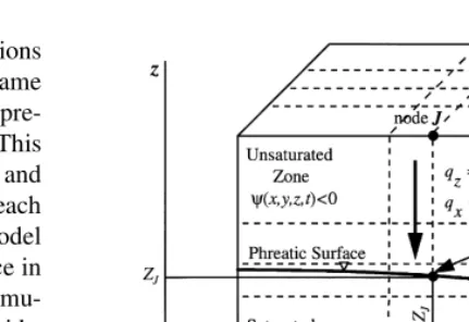
Figure 1 depicts a schematic view of the modeled hydro-logic system which includes both the unsaturated and the underlying saturated zone. The motion of water in the unsaturated–saturated zone of the soil can be simulated by the 3-D Richards equations,1i.e.
]v
]t¼=· K·=ðwþzÞ
þI (1)
wherevis the soil water content,w is the matric pressure head,K is the hydraulic conductivity tensor,z is the ver-tical coordinate (positive upward),Iis a sink-source term, andt is time.
Let us introduce the following simplified assumptions: (1) the flow in the unsaturated zone is in the vertical direction
only; (2) the Dupuit assumption of essentially horizontal flow is valid in the saturated zone; (3) water is practically incompressible, its density does not depend on solute con-centration; (4) the porous matrix is rigid.
The equation that describes the phreatic surface reads
h xÿ ,y,t
¹z¼0 (2)
wherehis the elevation of the phreatic surface,xandyare the planar coordinates.
In the unsaturated zone the model is presented by series of 1-D Richards equations evaluating vertical flow at points throughout an areal plane, i.e.
]v
]t¼ ]
]z Kzz ]w
]zþKzz
þI (3)
whereKzz is the vertical component of the hydraulic con-ductivity tensor.
The 2-D averaged flow equation for the saturated zone can be obtained by integrating the 3-D flow equation over the vertical direction.1 Following the assumption of rigid matrix, we note that in the saturated zone ]v=]t¼0, this
yields
Zhðx,y,tÞ
hðx,yÞ
=·qþI
ÿ
dz¼0 (4)
wherehis the elevation of the bottom of the aquifer andq
is the specific water flux vector. By employing Leibnitz rule we write eqn (4) in the form
=9·(h¹h)q˜9þqlh¹·=(z¹h)¹qlh¹·=(z¹h)þI˜¼0 (5)
where
˜
q9¼ 1
h¹h Zh
hq
9dzandI˜¼
Zh
hIdz
in which ()9denotes a property defined only in thexy-plane. The qlh¹ and qlh¹ denote the water flux vectors at the phreatic surface and at the aquifer bottom, respectively. Following Darcy’s law and Dupuit’s assumption1
˜
q9¼ ¹K9·=9h (6.1)
Fig. 1.Idealization of the modeled subsurface system with a
Taking into account that the normal fluxes at both sides of the phreatic surface eqn (2) are equal, we write2
¹Kzz In a similar manner at the aquifer bottom, we obtain
qlh¹·=(z¹h)¼qlhþ·=(z¹h) (6.3) where water flux through the bottom of the aquifer,qlh¹, can be either prescribed, or calculated using known head values at the top of the underlying confined aquifer.1
The last term in eqn (5) we present in the form
˜
where Pw is the rate of the flux source/sink located at a
point (xl,yl) anddis the Dirac delta function. In view of eqn
The position of the moving phreatic surface is evaluated by
wÿx,y,z,t
As a result, we decompose the 3-D flow problem to a 1-D vertical direction presented by eqn (3) for the unsaturated zone, and to a 2-D horizontal plane for the saturated zone presented by eqn (7). We note, that eqn (7) refers to a nonsteady state, since ]w=]z andh are functions of time,
i.e time is included in eqn (7) implicitly as a parameter. Boussinesq equation for a leaky–phreatic aquifer is given by1
whereSy is the specific yield and Nis the natural replen-ishment (from precipitation and/or artificial recharge).
The main difference of eqn (7) from eqn (9), is that the first does not contain a storage term with specific yield and a source term for natural replenishment. Instead it explicitly models a vertical flux term at the phreatic surface. In view of eqn (7), the source term in eqn (9), reads
N¼Sy
Hence, the natural replenishment depends on the specific yield of the phreatic aquifer. We can also see from eqn (10)
that Nis equal to the Darcy flux only for steady state flow conditions.
Pikul et al.13 used 1-D Richards equation to simulate vertical flow in the unsaturated zone and 1-D form of eqn (9) to simulate horizontal flow in the saturated zone. Two parameters S(x,t) and N(x,t) were adjusted for each time step. TheSparameter was calculated as a response to the change of water content due to the water table move-ment, while the N parameter was found from the mass balance at every vertical line of the finite difference grid. As was noted by Vachaud and Vauclin,20such an approach is physically incorrect and the use of a linked system of equations resting on the concept of a storage coefficient may not yield simplification. Unlike this, in our model, eqn (3) is linked with eqn (7) by the flux term on the left hand side of eqn (7), and by eqn (8). Thus, our model does not require an introduction of the additional storage parameter.
The transport of contaminant species is described by the advection–dispersion equation.1 Here, for the sake of simplicity, we consider one conservative solute component in the soil water without any reaction with the solid matrix, i.e.
whereCis the concentration of the solute in the soil water,
Dis the apparent dispersion tensor,Cp
I is the concentration
of the solute in the injected water, andHis the Heaviside step function.
Initial conditions at timetodescribe the distribution in the soil of the matric potential (assumed to follow hydrostatic pressure in the saturated zone), the groundwater level, and the solute concentration.
The boundary conditions for eqn (3) at the soil surface (z¼Zs) can be given in the form
whereqsis the water flux at the soil surface, and the con-dition (8) at the phreatic surface (z¼h).
The plane boundary conditions for eqn (7) can be written in a general form, as
¹ K9ÿh¹h
where G9 represents the plane boundary, and bhG9 is a
parameter which defines the type of the boundary condi-tion,nis a unit vector normal to the boundary,hG9 andQG9
are prescribed head and flux values, respectively.
In a similar fashion, the boundary condition for the trans-port equation, eqn (11), reads
¹Dv·=C¹qC·nþbCG C¹CG
ÿ
¼QCG x[G
whereGrepresents the space boundary,bCG is a parameter
which defines the type of the boundary condition,CG and
QCG are the prescribed concentration and the solute flux
values, respectively.
3 NUMERICAL ALGORITHM
In what follows we describe a general algorithm to solve the flow problem eqns (3), (7) and (8) together with the trans-port problem eqn (11), in a 3-D space. To investigate the performance of the algorithm, we implemented it to a com-puter code for quasi 2-D cross-sectional problems which was verified against the simulations of fully 2-D variably saturated flow and transport of other codes.
To solve eqns (3), (7), (8), () and (11), we implement a finite difference grid in a 3-D space (Fig. 1). We solve the 1-D Richards eqn (3) along the vertical coordinatezof everyJnodal point situated at (xj,yj) on the horizontal plane. The right hand side (r.h.s) of eqn (7) is approximated by finite difference on the horizontal section of the 3-D grid.
The solution algorithm is described as follows:
(1) Use the prescribed distribution of the capillary pressure headwJ z,tk
ÿ
of the previous time leveltk(or pre-vious iteration) at each nodeJ, to find the heightZJat which w ZJ,tk
ÿ
¼0. This can be found by applying a linear inter-polation formula between nodesziandziþ1, along the same vertical (in a nodeJ), wherewi.0 andwiþ1,0, respec-heightZJ, constitutes the location,hJ, of the phreatic surface for every nodeJ, i.e.hJ(xJ,yJ,tk)¼ZJ(Fig. 1).
(2) Calculate the r.h.s. of eqn (7) at each nodeJusing its finite difference approximation. A standard finite difference scheme is used. To deal with aquifers where the perme-ability varies in the vertical direction, we substitute
K9ÿh¹h
At the plane boundary nodes, the r.h.s of eqn (7) is calcu-lated with its appropriate boundary condition eqn (13). Note, that ifbhG9¼`, we obtain from eqn (13) the Dirichlet
boundary conditionh¼hG9. In this case there is no need to
calculate the r.h.s of eqn (7), that is, the Dirichlet condition is implemented directly at the low boundary for the 1-D Richards equation.
The value defined by the r.h.s of eqn (7) constitutes the flux in the unsaturated zone at the phreatic surface. For eqn (3) we have a typical problem with a moving lower boundary defined by eqn (7). To simplify the solution, we implement eqn (7) as the boundary condition instead of eqn (8), and project eqn (7) from the phreatic surface to the bottom of the aquifer, or to some plane level below the phreatic surface. This can be done artificially, since the vertical component of Darcy’s velocity is constant in
the saturated zone, when considering the 1-D Richards equation. Indeed, on one hand, we have eqn (7) at the phrea-tic surface which is moving. On the other hand, assuming that the water is incompressible and the solid matrix is rigid, we obtain for the 1-D vertical flow in the saturated zone
]=]zKð]w=]zþ1Þ
¼0. Hence, Kð]w=]zþ1Þ ¼ const for
anyzbelow the phreatic surface. Thus, we replace the pro-blem of solving Richards equation with a moving lower boundary with one with a fixed boundary. Note, that the actual value of the normal flux through the aquifer bottom is of course different from eqn (7), it is defined by equation (6.3).
(3) Given the boundary condition eqn (12) at the soil surface, solve for wÿz,tkþ1
using eqn (3). An implicit mass conservative scheme,4 based on the mixed form of the Richards equation is used for the finite differences approximation of eqn (3).
(4) Evaluate the vertical component of Darcy’s velocity in the unsaturated zone and two horizontal components of Darcy’s velocity in the saturated zone, at thetkþ1time level. The horizontal components of the water flux in the unsatu-rated zone are equal to zero. The vertical component of the water flux in the saturated zone can be approximately evalu-ated by integrating the water balance equation,14,16 while the horizontal fluxesq˜9, in that equation, are prescribed by
equation (6.1), i.e.
whereAis a constant which can be found using the value of the water flux at the bottom of the aquifer.
(5) Solve the three-dimensional transport problem eqn (11), at the tkþ1 time level, through the unsaturated and the saturated zones.
Since eqns (3), () and (7) are nonlinear, a simple iterative procedure is used for their solution until a desired degree of convergence is achieved throughout the entire domain. The iterative procedure is applied to both equations simulta-neously. However, since the water level (h) is equal to the potential head (F;wþz¼h) forz¼h, the convergence criteria is checked only for the pressure head (w) values. During simulations, time step is changed between pre-scribed minimum and maximum values. At any time level, the time step is automatically adjusted by multiplying a predetermined constant. The latter is greater than a unit if the number of iterations necessary to reach convergence less than that of a prescribed one. If at some time level the number of iterations becomes greater than a prescribed maximum, the time increment is decreased and the itera-tions are restarted for this time level.10
At each iteration, eqn (7) is not solved directly, since its r.h.s explicitly defines a flux at the phreatic surface. Yet, theh values are found at any nodeJby interpolation, using the solution forwJðz,tÞfrom the previous iteration as is described in ref.1. Theseh are then substituted into eqn (7).
unsaturated hydraulic conductivity we refer to the van
tent,vsis the water content at saturation,Ksis the saturated hydraulic conductivity of the soil, a and n are Van Genuchten model parameters, andm¼1 ¹1/n.
We note that the 3-D formulation for flow and transport in the unsaturated–saturated medium is presented by eqns (1) and (11). The quasi 3-D formulation for these problems is given by eqns (3), (7), (8) and (11). At this stage, we have conformed the quasi 3-D formulation and the solution algorithm to deal with quasi 2-D cross-sectional problems. This was implemented to a computer code (QUASI2D) aimed at simulating 2-D flow and transport in an unsaturated–saturated media. The performance of QUASI2D was therefore compared against 2-D variably saturated models based on the solution of the 2-D Richards equation and the transport equations. This will help to reveal the model limitations and the drawbacks of the presented algorithm. The implementation of the model for more general quasi 3-D cases will be reported in a sequel paper.
When referring to the quasi 2-D cross-sectional case, the formulation can be further simplified. We recall, that water flow in the unsaturated zone is only vertical, while in the saturated zone it is essentially horizontal. Therefore, we consider, for the quasi 2-D case, these two directions as the principal axes of the dispersion, i.e. Dxz ¼ Dzx ¼ 0. The two remaining components of the dispersion tensor are given by1
Dxx¼Dmtcþ(aTVz2þaLVx2)=V and
Dzz¼Dmtcþ(aLVz2þaTVx2)=V ð18Þ
whereDm is the molecular diffusion coefficient, tc is the tortuosity factor, aL and aT are the longitudinal and the transverse dispersivities of soil, respectively, Vx,, Vz and
V (¼ V2
xþVz2
p )
are the horizontal and vertical compo-nents of the average water velocity vector and its module, respectively.
Multiplying the water mass balance eqn (1) by C and subtracting it from eqn (11), we obtain for the 2-D case
v]C
Since eqn (19) does not contain terms with cross-derivatives, we can use the operator splitting method15 to solve a 2-D transport equation. According to this method, eqn (19) can be split into two sequential one-dimensional
parts
is the finite difference operator approximating the diffusion and advection parts in the r.h.s. of eqn (19). The monotone scheme15 was used to approximate eqn (20) on a finite difference grid.
At every time leveltkþ1, eqn (20) can be written in eachz direction at a nodeias
vkiþ1=2
whereÉziis the grid step along coordinatezassociated with
a nodei, and
In eqn (21), the space derivatives, representing the advec-tive solute flux in eqn (19), are automatically approximated by upstream finite difference. This dictates a monotone scheme which ensures a solution without oscillations. The introduction of a parameter q gives an approximation of order O(É2)in space for the whole scheme eqn (21).15The approximation in time is of first order.
Approximating also the boundary condition eqn (14), the set of the linear algebraic equations can be solved, e.g. by Thomas algorithm.
4 MODEL VERIFICATION FOR THE QUASI 2-D CASE
transport in the unsaturated and saturated zones, we com-pared the model’s quasi 2-D predictions with those obtained by a 2-D variably saturated flow and transport equations which were simulated by the 2DSOIL10,18 and the SUTRA22numerical (finite element) models. The 2DSOIL code is partially based on the code SWMS_2D developed by Simuneket al.17 SUTRA is a code for simulation of fluid density dependent flow, and iterations procedure are exe-cuted for both the flow and the transport equations at each time step. Since we do not consider problems of density dependent flow and to reduce the computation time, the iterations for the transport equation in SUTRA were ‘frozen’. Three synthetic examples were considered.
4.1 Example 1. Spread of a groundwater ‘stripe’
The groundwater level at the initial time, t0, is given as a step function
h(x,t0)¼
h0 if lxl$R
h0þDhiflxl,R
(
(22)
whereh0and the stepDh3Rare prescribed. The analytical solution of the linearized 1-D Boussinesq equation for this case, has the form14of
h(x,t)¼h0þ Dh
2 erf
R¹x
2patþerf Rþx
2pat
!
(23)
where a¼Ks=(Syh˜), Sy is the specific yield and h˜ is the
average groundwater level.
We carried out simulations for the silt loam GE 3 soil for which21vs¼0.369,vr¼0.131,Ks¼0.0496 m per day,a¼ 0.423 m¹1 andn¼2.06. The longitudinal and transversal dispersivities were prescribed asaL¼1.0 m andaT¼0.1 m, respectively. The simulated domain was presented by a
rectangle of height 4 m (from bottom of the aquifer to the soil surface) and 40 m length. The assigned initial condi-tions wereh0¼2.0 m,Dh¼0.5 m, andR¼5.0 m. We note the symmetry of eqn (22) atx¼0. Hence, accordingly, the
]h/]x¼0 condition was assigned. No flow condition was
also specified at z ¼ 0 and z ¼ 4 m. At x ¼ 40 m, we prescribed a constant headh¼2 m. The initial solute con-centration was set to be C0 ¼ 1 for 0#x#R and
h0#z#h0þDh, andC0¼0 elsewhere. A finite difference grid of 17 3 17 nodes was used to solve the quasi 2-D problem. The steps of the grid were 2.5 m and 0.25 m along xandz coordinate axes respectively. An equivalent finite element grid (the same number of nodes at the same locations) was implemented for simulations with SUTRA and 2DSOIL. The time step was increased by a factor of 1.1 starting from 10¹6
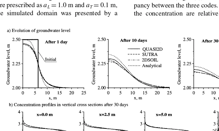
day. Simulation with QUASI2D regard-ing groundwater level, was between the analytical solution of the linearized Boussinesq equation and the numerical solution of the 2-D Richards equation, however, closer to the latter one (Fig. 2(a)). This is due to the fact that the quasi 2-D model accounts for both the specific features of the variable saturation model and for the limitations of the Dupuit assumption. The maximum difference was 3 cm at the groundwater summit (x¼0), where QUASI2D predicts higher groundwater level than the fully 2-D model, since the first does not account for the horizontal water flux in the capillary fringe. The simulated distribution of the water content in the unsaturated zone was in good agreement with the one obtained on the basis of the 2-D Richards equation. The maximum difference between QUASI2D, 2DSOIL and SUTRA did not exceed 0.002 cm3cm¹3
. The concentrations obtained by the quasi 2-D approach and the fully 2-D flow and transport, compare well for x¼0, 2.5 and 5.0 m (Fig. 2(b)). Forx¼7.5 m there is a discre-pancy between the three codes. However, absolute values of the concentration are relatively small there. Figure 2(b)
demonstrates that SUTRA produces oscillatory solution in the last cross-section.
The computation time, for the period of 30 days, using QUASI2D, 2DSOIL and SUTRA is presented in Table 1. We note that the QUASI2D code was several times faster than the 2DSOIL and SUTRA codes.
4.2 Example 2. Infiltration from the soil surface
A problem of time dependent water infiltration and solute transport through the soil surface was considered. The simu-lations were carried out for the Guelph loam soil for which21 vs ¼ 0.520, vr ¼ 0.218, Ks ¼ 0.316 m per day, a ¼ 1.15 m¹1,n ¼ 2.03. The longitudinal and transversal dis-persivities were set equal to aL ¼ 5.0 m and aT ¼1.0 m, respectively. The simulated domain was presented by a rectangle of height 10 m (from bottom of the aquifer to the soil surface) and 300 m length. Initial groundwater level wash0¼4 m. Initial solute concentration was equal to zero. Water flux was assigned at the soil surface for the segment 110 , x , 170 m. During the first 3 years, the intensity of the flux was 2 mm per day with a concentration of the solute in the water equal to 1; during the next 3 years, these were 0.2 mm/day and 0, respectively; and during the last 4 years, a no flow condition was implemented. The boundary conditions h ¼ 4.0 m for flow and C ¼ 0 for transport, were specified at x¼ 0 m. The remaining part was subject to no flow boundary condition. A finite differ-ence grid of 16318 nodes was used to solve the quasi 2-D problem. A constant grid step equal to 20 m was assigned along thexcoordinate, the grid step along thezcoordinate increased from 0.25 m at the soil surface to 1 m at the bottom of the aquifer. An equivalent finite element grid was implemented for simulations with SUTRA and 2DSOIL. The time step increased by a factor of 1.5 starting from 10¹6
day. The maximum value of the time step was 10 days. Simulation with QUASI2D regarding groundwater level, was closer to the one obtained by the 2DSOIL code (Fig. 3). Again, as in the case of Example 1, QUASI2D slightly overestimates the groundwater level at its summit (Fig. 3, after 3 years). The simulated distribution of the water content in the unsaturated zone was consistent with the one obtained on the basis of the 2-D Richards equation. The maximum difference in water content for three codes did not exceed 0.01 cm3cm¹3
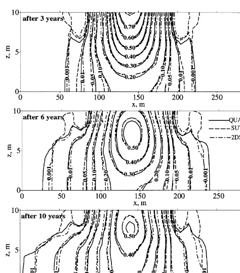
. The contours of concentra-tion, obtained by the quasi 2-D approach and the fully 2-D flow and transport, were also very similar (Fig. 4). However, SUTRA again produced oscillation and negative concentra-tion values in the vicinity of the concentraconcentra-tion front.
The computation time for QUASI2D was less in compari-son to 2DSOIL and SUTRA (see Table 1).
4.3 Example 3. Infiltration from the soil surface and internal water sink
In this example we consider the problem of constant water infiltration through the soil surface and internal water sink. The flow domain is depicted in Fig. 5. The flow domain is heterogeneous and composed of three types of soil: (1) Touchet silt loam soil for which21vs¼0.469,vr¼0.190,
Ks ¼3.03 m per day, a ¼ 0.5 m
¹1
, n ¼ 7.09, the longi-tudinal and transversal dispersivities wereaL¼40.0 m and
aT¼2.0 m, respectively; (2) Guelph loam soil for which21 as ¼ 0.520, vr ¼ 0.218, Ks ¼ 0.316 m per day, a ¼ 1.15 m¹1,n¼2.03, the longitudinal and transversal disper-sivities wereaL¼60.0 m andaT¼3.0 m, respectively; (3) Sand for which8vs¼0.340,vr¼0.0055,Ks¼5.66 m per day, a ¼ 4.18 m¹1
,n ¼2.19, the longitudinal and trans-versal dispersivities were aL ¼ 30.0 m and aT ¼ 1.0 m,
Table 1. Computation time (CT, s), number of time steps (NS) and computation time per step (TS, s) using a Pentium/120 PC
Example 1 Example 2 Example 3
Code CT NS TS CT NS TS CT NS TS
QUASI2D 7 176 0.040 15 412 0.036 240 3587 0.067 SUTRA 68 164 0.415 168 388 0.433 1180 1490 0.792 2DSOIL 60 164 0.366 145 388 0.374 1090 1490 0.732
Fig. 3.Groundwater level during infiltration from the soil surface
respectively. Initial groundwater level was equal to 45 m, initial solute concentration was equal to zero. Water flux was prescribed at the soil surface for the segment 2050,
x, 2450 m. The intensity of the flux was 5 mm per day with the concentration of the solute in the water equal to 1, during 20 years. The boundary conditionsh¼45 m for flow andC¼0 for transport, were specified atx¼3000 m. The remaining part of the boundary was subject to a no flow condition. A constant rate of water uptake by the internal linear sink was 1.5 m2per day. A finite difference grid of 31318 nodes was used to solve the quasi 2-D problem. A constant grid step equal to 100 m was assigned along thex
coordinate, the grid step along the zcoordinate increased from 0.5 m at the soil surface to 5 m at the bottom of the
aquifer. An equivalent finite element grid was implemented for simulations with SUTRA and 2DSOIL.The time step increased by a factor of 1.5 starting from 10¹6
day. The maximum value of the time step was 5 days.
Figure 6 presents the simulated groundwater level after the 20 years period. The phreatic surface, calculated on the basis of QUASI2D, is situated between phreatic surfaces obtained by SUTRA and 2DSOIL. The maximum differ-ences of groundwater level are 20 cm atx,500 m between QUASI2D and 2DSOIL, and 14 cm atx.1200 m between QUASI2D and SUTRA. The maximum difference between SUTRA and 2DSOIL is 26 cm. The maximum difference for the water content in the unsaturated zone simulated on the basis of QUASI2D and on the basis of the 2-D Richards equation, did not exceed 0.015 cm3cm¹3
.
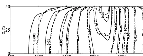
Figure 7 depicts the contours of concentration profiles at different cross-sections after 20 years. The agreement between the QUASI2D and the variable saturation models is worse than in the two previous examples. This is most pronounced in the direction of the flow towards the sink. Comparing the 0.5 contour lines in this direction, we note that the concentration front simulated by QUASI2D is smoother than that obtained by SUTRA and QUASI2D. Since the flow regimes predicted by the models were very similar, the differences in concentration values result mainly from the different numerical schemes for solving the transport equation. This, will be discussed in the follow-ing section.
The computation time, for the total period of 10 years, was again less for QUASI2D, in comparison to 2DSOIL and SUTRA (see Table 1).
5 DISCUSSION
We note (Table 1), that in all three examples the computa-tion time of QUASI2D was much smaller in comparison to that of SUTRA and 2DSOIL. This efficiency can be explained on the basis of using the quasi 2-D model to solve for the series of 1-D problem. The resulting smaller set of approximating algebraic equations yield a much less computational effort. It is also evident from Table 1 that the computation time of SUTRA is higher in comparison to
Fig. 4.Contours of solute concentration during infiltration from
the soil surface (example 2).
2DSOIL. Both SUTRA and 2DSOIL solve for eqns (1) and (11) in their 2-D formulation. The SUTRA algorithm employs hybrid finite element and integrated finite differ-ence method, using quadrilateral elements and bi-linear basis function, while the 2DSOIL model is based on the finite element solution using triangular and/or rectangular elements and linear bases functions. An implicit scheme was implemented to both codes with a first order approxi-mation in time and of second order in space. Yet, SUTRA’s numerical algorithm is not specifically aimed at dealing with nonlinearities of unsaturated flow as would be required of a model simulating only unsaturated flow.22The 2DSOIL code has the ability to adjust the iteration domain to that where convergence criteria are not met, and it also has a table look-up function of water content and hydraulic con-ductivity as a function of matric pressure head. These enables a faster solution. Simulations have shown that all three codes perfectly conserved water mass balance.
The maximum time steps for the considered examples was chosen so that the solution for the pressure head will converge when solving a fully 2-D flow. The SUTRA code stops the computation due to non convergence of pressure for large time steps, while 2DSOIL and QUASI2D decrease automatically the time step in such a case. In all three examples, SUTRA and 2DSOIL attained the maximum time step which then remained constant until the end of the simulation period.
Table 1 demonstrates that in each simulation, the QUASI2D code performed more time steps than SUTRA and 2DSOIL. Hence, the actual sizes of time step achieved by QUASI2D were smaller from the prescribed maximum time step. An attempt to increase the time step for QUASI2D led to oscillation of the head values and to non convergence of iterations for the flow problem. Such non stable behavior was due to the explicit scheme of the coupling between eqns (3) and (7). To explain this, let us consider a simple situation. Suppose that at some time we have a gradient of groundwater level between any two neighboring points in the plane (Fig. 8(a)). The low bound-ary fluxes,Q01andQ02, calculated at these points for Richards equation, are explicitly defined by the r.h.s. of eqn (7) and they depend on the gradient of water level. Water flowing from the point with the higher groundwater level to the point with the lower one, decreases the water level at the first point and increases it at the second point. If the time step is large enough, then after the first iteration, we can get a
situation when the calculated gradient of groundwater level changes its direction (Fig. 8(b)) and it might be steeper than the initial gradient. Next iteration will change the direction of the water level gradient to the initial (Fig. 8(c)). Con-tinuing iterations increases the oscillations amplitude and blows up the solution. This effect is most significant when the gradient of the water level is more than 0.01. Actually, when we have infiltration on the phreatic surface and inter-nal sink-sources, the situation is even more complicated than in the considered example. Another reason for a non convergent solution can be due to round off errors when calculating the position of the phreatic surface and the r.h.s. of eqn (7). An attempt to change the QUASI2D algo-rithm by solving directly eqn (7) with the flux term taken from the previous iteration, did not improve the solution regarding its convergence for large time steps, while it increased the time of computation. Therefore, to obtain a convergent solution, we used a simple procedure of time and iteration control as was described in Section 3.
As a general remark, let us note that the model presented by eqns (3), (7) and (8), can be considered as a typical free boundary problem. The instability of the solution is a central question in such problems. Its investigation involves signi-ficant difficulties even for linear cases. A detailed review of this question was given by, e.g. Langer.7For the model eqns (3), (7) and (8), this can be a subject of a separate study in future.
The computational efficiency per time step of the codes is presented in Table 1. In the examples 1 and 2 (number of nodes 289 and 288, respectively), QUASI2D was 10 and 13 times faster in comparison to SUTRA and six and seven times faster in comparison to 2DSOIL. In example 3 (number of nodes 558) the computation time per one step of QUASI2D was 22 and 16 times faster in comparison to SUTRA and 2DSOIL, respectively.
As was mentioned above, in the considered three examples, QUASI2D produced a concentration front which was smoother than the one simulated by SUTRA and 2DSOIL. This can be explained by the application of the monotone finite difference scheme eqn (21) on a coarse grid for non-conservative form of the transport eqn (19). This scheme does not allow oscillation by introducing
Fig. 7.Contours of solute concentration after 20 years (example 3).
Fig. 8.Scheme illustrating non convergent solution for large time
some artificial dispersion of order O(É2). As was evident in the presented examples, the coarser the space grid, numeri-cal dispersion increased in the direction of flow when using the monotone scheme for the transport equation. We also noticed that SUTRA yielded small negative concentration values and oscillation, while 2DSOIL produced ‘overshoot-ing’ at some cross sections (not shown). Non-monotone behavior of the numerical solution of the advection– dispersion equation is a function of the Peclet, Courant numbers and the temporal (e.g. fully-implicit, fully-explicit and Crank–Nicholson) as well as spatial (e.g. upstream, central, flux limiting) weighting schemes.12,19In the simu-lations, we used a fully-implicit scheme which is uncondi-tionally stable. The Courant number (Crz¼lqzlt=Éz,
z¼1,2) did not exceed 0.8 in the entire domain. Therefore, we can conclude that the problem of oscillation emerged from the approximation of the advective flux term of the transport equation. The simplest way to overcome the ‘over-shooting’ or ‘under‘over-shooting’ problem is to superimpose some relations between dispersion parameters and the grid sizes. For example, the following inequalities should be approximately satisfied:22 Éx#4aL and Éz#10aT.
Although these conditions were introduced in our examples, the oscillation problem still remained. Another way to pos-sibly circumvent the numerical oscillations is to use the upstream weighting. The SUTRA algorithm can use the asymmetric weighting function which adds artificial disper-sion related to the element size.22 In a similar way the 2DSOIL code has the possibility of weighting the advective flux term by nonlinear functions.17,23 We made additional simulations using the aforementioned upstream weighting schemes, however this did not improve the results in terms of numerical oscillations.
The solution of the transport equation in the conservative form eqn (11) gives better mass balance than the solution of eqn (19). The solute mass was almost fully conserved by SUTRA and 2DSOIL. The conservation of solute by QUASI2D was with an error less than 0.5% of the total mass of the solute in examples 1 and 2, while in example 3 it produced an error of 4%.
6 CONCLUSION
Simulations for the quasi 2-D case proved to be computa-tionally very efficient for the modeling of field scale flow and transport in the unsaturated and saturated zones. It can, therefore, be speculated that it will even be more efficient in comparison to fully 3-D unsaturated–saturated flow and transport models.
The advantage of the developed algorithm for the flow problem, is that we actually solve only a set of 1-D Richards equations at each time step. The possible instability of the solution for large time steps represents the major drawback of this algorithm.
Let us also to point out some limitations of a quasi 3-D approach. The quasi 3-D model cannot be implemented for
simulation of water flow and solute transport from a point source in the unsaturated zone (e.g. drip irrigation). In such cases the horizontal water fluxes can be significant. We also note that the quasi 3-D model does not account for the horizontal water fluxes in the capillary fringe, which can be relatively important, mainly with shallow water table aquifers of small thikcness.20 Since this model is based on Dupuit’s assumption, it can be applied to aquifers with small gradient values of the phreatic surface, while at the vicinity of outlets or wells its solution may be misleading. For a multiaqifer system, the quasi 3-D model for the upper phreatic aquifer can be coupled with the quasi 3-D model of the underlying confined aquifers.
ACKNOWLEDGEMENTS
Thanks are attributed to the Rashi Foundation for the financial support that was provided to conduct this research.
REFERENCES
1. Bear, J. and Verruijt A., Modeling Groundwater Flow and Pollution. D. Reidel, Dordrecht, 1987.
2. Borisov, V. S. and Manukian D. A. Simulating of water and salt regime of soil when designing systems of irrigation. In Automatic Preparation and Management in Water Engineering, ed. V. Voropaev, VNIIGiM, Moscow, 1985. pp. 110–119 (in Russian).
3. Bredehoeft, J. D. & Pinder, G. F. Digital analysis of areal flow in multiaquifer groundwater system: A quasi-three-dimensional model.Water Resour. Res., 1970,6,883–888. 4. Celia, M. A., Bouloustat, E. T. & Zabra, R. L. A general
mass-conservative numerical solution for the unsaturated flow equation.Water Resour. Res., 1990,26,1483–1496. 5. Herrera, I. & Rodarte, L. Integrodifferential equations for
systems of leaky aquifers and applications. 1. The nature of approximate theories. Water Resour. Res., 1973, 9, 995– 1005.
6. Kool, J. B., Huyakorn, P. S., Sudicky, E. A. & Saleem, Z. A. A composite modeling approach for subsurface transport of degrading contaminants from land disposal sites.J. Contam. Hydrol., 1994,17,69–90.
7. Langer, J. S. Instabilities and pattern formation in crystal growth.Rev. of Modern Physics, 1980,52,1–28.
8. Mishra, S., Parker, J. C. & Singhal, N. Estimation of soil hydraulic properties and their uncertainty from particle size distribution data.J. Hydrol., 1989,108,1–18.
9. Neuman, S. P., Preller, C. & Narasimhan, T. N. Adaptive explicit–implicit quasi three-dimensional finite element model for flow and subsidence in multiaquifer systems. Water Resour. Res., 1982,18,1551–1561.
10. Pachepsky, Ya., Timlin, D., Acock, B., Lemmon, H. and Trent A., 2DSOIL—A new modular simulator of soil and root processes. USDA-ARS, System Research Lab., Belts-ville MD, 1993.
12. Perroschet, P. & Berod, D. Stability of the standard Crank– Nicholson–Galerkin scheme applied to the diffusion– convection equation: Some new insight. Water Resour. Res., 1993,29,3291–3297.
13. Pikul, M. F., Street, R. L. & Remson, I. A numerical model based on coupled one-dimensional Richards and Boussinesq equations.Water. Resour. Res., 1974,10,295–302. 14. Polubarinova-Kochina, P.Ya., Theory of Groundwater
Motion. Nauka, Moscow, 1977 (in Russian).
15. Samarsky, A.A., Theory of Finite Differences Schemes. Nauka, Moscow, 1977, pp. 656 (in Russian).
16. Strack, O. D. L. Three dimensional streamlines in Dupuit– Forchimer models.Water. Resour. Res., 1984,20,812–822. 17. Simunek, J., Vogel, T. and M. van Genuchten, The SWMS_2D code for simulating water flow and solute trans-port in two-dimensional variably saturated media. Version 1.1., Research Report No. 126. US Salinity Lab, 1992, pp. 169. 18. Timlin, D. & Pachepsky, Ya. A modular soil and root process
simulator.Ecological modeling, 1997,94,67–80.
19. Unger, A. J. A., Forsyth, P. E. & Sudiky, E. A. Variable
spatial and temporal weighting schemes for use in multi-phase compositional problems. Adv. Water Resour., 1996,
19,1–27.
20. Vachaud, G. & Vauclin, M. Comments on ‘A numerical model based on coupled one-dimensional Richards and Boussinesq equations’ by Mary F. Pikul, Robert L. Street, and Irwing Remson.Water. Resour. Res., 1975,11,506–509. 21. van Genuchten, M.T. A closed form equation for predicting the hydraulic conductivity of unsaturated soil.Soil Sci. Soc. Am. J., 1980,44,892–898.
22. Voss, C. I., A finite-element simulation model for saturated– unsaturated, fluid-density-dependent ground-water flow with energy transport or chemically-reactive single-species solute transport, US Geol. Surv. Water Resour. Investig. Report No. 84-4369, Reston VA, 1984.