Uncertainty and equifinality in calibrating
distributed roughness coefficients in a flood
propagation model with limited data
G. Aronica
a ,*, B. Hankin
b& K. Beven
b aDipartimento di Ingegneria Idraulica e Applicazioni Ambientali, Universita` di Palermo, Viale delle Scienze, 90128 Palermo, Italy b
Institute of Environmental and Natural Sciences, Lancaster University, Lancaster LA1 4YQ, UK
(Received 1 September 1997; revised 7 May 1998; accepted 27 May 1998)
Monte-Carlo simulations of a two-dimensional finite element model of a flood in the southern part of Sicily were used to explore the parameter space of distributed bed-roughness coefficients. For many real-world events specific data are extremely limited so that there is not only fuzziness in the information available to calibrate the model, but fuzziness in the degree of acceptability of model predictions based upon the different parameter values, owing to model structural errors. Here the GLUE procedure is used to compare model predictions and observations for a certain event, coupled with both a fuzzy-rule-based calibration, and a calibration technique based upon normal and heteroscedastic distributions of the predicted residuals. The fuzzy-rule-based calibration is suited to an event of this kind, where the information about the flood is highly uncertain and arises from several different types of observation. The likelihood (relative possibility) distributions predicted by the two calibration techniques are similar, although the fuzzy approach enabled us to constrain the parameter distributions more usefully, to lie within a range which was consistent with the modellers’ a priori knowledge of the system.q1998 Elsevier Science Limited. All rights reserved
Keywords: flood inundation models, roughness coefficient, parameter calibration, likelihood, fuzzy logic, fuzzy rules.
1 INTRODUCTION
The principal purpose of this paper is to compare two frameworks for the calibration and interpretation of the pre-dictions of a flood model of a real event, in an extremely complex system, on the basis of highly limited measure-ments. The generalized likelihood uncertainty estimation (GLUE) procedure9 is used here together with a fuzzy measure of the acceptability of different possible model structures and parameter sets. This is achieved by mapping the parameter space, via multiple model simulations, to the unidimensional space of a performance measure or objec-tive function, which expresses our relaobjec-tive degree of belief that the parameters provide a model structure which is a good simulator of the system.
The application of this fuzzy calibration technique represents a new paradigm in the way we interpret predic-tions of physically based models, which moves away from parameter optimization techniques which tend to imply that the structure of the model can be precisely determined. In general, there will be a degree of ambiguity, or non-random uncertainty associated with the data and the structure of the model, which is exposed if we view all the predictions relativistically. There is much to recommend the fuzzy calibration technique as a general approach to modelling such complex systems, particularly where, as here, the data set available for calibration is very limited.
In this study of the flood in the Imera Basin, the friction resulting from floodplain and river channel roughness are considered to be the most important parameters controlling the large scale flow characteristics6,20. The initial stage of this study, in which Monte Carlo simulations of the flood event are made using different values for the roughness
Printed in Great Britain. All rights reserved 0309-1708/98/$ - see front matter PII: S 0 3 0 9 - 1 7 0 8 ( 9 8 ) 0 0 0 1 7 - 7
349
coefficients, is similar to the investigation made by Bates
et al.7. The authors report finding many different parameter values giving rise to equivalent model simulations, in terms of objective function values. This non-identifiability of roughness parameter values highlights the need to avoid reliance upon parameters, which were optimized at the calibration stage. Data errors, choice of objective function and the flow characteristics for any particular study5 can affect optimized parameters. The GLUE procedure seeks to allow for these problems, by placing emphasis on the study of the range of parameter values, which have given rise to all of the feasible simulations.
The GLUE procedure has previously been used by Romanowicz et al.20to produce flood risk maps on a section of the River Culm from a simple flood routing model based around the concept that in such extreme events, flow control is dominated by frictional and gravitational effects. In her study, the output from the simple flow model was calibrated against the simulated results of a finite element flood model6. This first approach provided the simple model with unrealistically large amounts of calibration informa-tion and was next developed to be based on maximum inundation information alone, which is more consistent with the information, which is usually available after a real event19. Both of these applications utilized a statistical error model for the distribution of predicted residuals in order to derive a likelihood measure.
In this paper, objective functions, which are based upon both fuzzy and statistical frameworks, are used to provide likelihood measures, which can at later stages be used to express the uncertainties in model predictions, via the GLUE procedure. These measures will be referred to as likelihoods throughout, although these should be understood to represent ‘relative possibility measures’ to avoid any confusion with orthodox definitions of likelihood functions. The formulation of model predictions in a possibilistic framework is considered, the ultimate aim being to use this information to derive percentile risk maps for inundation in flood events in a GIS framework.
It is suggested here that where the information available to constrain the modelled system is limited and where it is derived from observations of different variables, it would be more easily incorporated by using objective functions which are based on fuzzy rules. Further, fuzzy rule based constraints can be made to be less stringent, which can help to avoid situations in which the system is falsely over-constrained.
2 THE HYDRODYNAMIC MODEL
The mass and momentum conservation equations for two-dimensional shallow-water flow, when convective inertial terms are neglected, can be written as follows:
]H
q(t,x,y) are the x and y components of the unit discharge
(per unit width), h is the water depth, Jx and Jy are the hydraulic resistances in the x and y directions. If Manning’s formula is adopted, the last terms in eqns (1b) and (1c) can be expressed as:
where c is Manning’s roughness coefficient.
2.1 Numerical solution of the Saint-Venant equations
Eqns (1) are solved by using a finite element technique with triangular elements. The free surface elevation is assumed to be continuous and piece-wise linear inside each element, where the unit discharges in the x and y directions are assumed to be piece-wise constant. The use of the Galerkin finite element procedure12,25 for the solution of eqn (1a) leads to:
where Ni¼Ni(x,y) are the Galerkin shape functions and n is the total number of the mesh nodes. The interpolation functions Hˆ , pˆ and qˆ are defined as:
where Hjis the free surface elevation at node j and peand qe are the unknown unit discharge components inside the
element e located around the point with coordinate vector components x and y.
Substituting eqn (4) into the governing eqn (3) and using Green’s formula for integration by parts yields:
Xne
where the integration is over the single element areaQe, cos
nx and cos ny are the direction cosines of the integration domain boundary L and ne is the total number of
elements.
From eqns (1b) and (1c) it is possible to obtain a unique relationship between unit discharges and free surface
elevations in the following discretized forms:
From eqns (6a) and (6b) it follows:
pkþ1¼ ¹E]H
The coefficient E, defined by eqn (8), is dimensionally homogeneous to a transmissivity and represents the unit discharge dispersion component per unit hydraulic gradi-ent. Substituting eqns (8), (9a) and (9b) into eqn (5) and assumingpˆ¼pkþ1, qˆ¼qkþ1, one can obtain: Eqns (10) form a linear set of n equations in the n unknowns Hkþ1, whose corresponding matrix is symmetric and positive definite. The solution of the system is easily obtained with the use of conjugate gradient methods. The integral terms in eqn (10) and eqns (11a) and (11b) are approximated by multiplying the coefficients E, Lx and
Ly, evaluated in the centre of element e, by the area of the same element. The unit discharges pkþ1 and qkþ1 can be thereafter computed by substitution of the free surface ele-vations Hkþ1into eqn (7). Finally, it is possible to enhance the stability of the time discretization scheme by changing the evaluation of the capacity term in eqn (11a) with the
following equation16:
that is equivalent to perform the ‘lumping’ of the time-dependent part of the matrix.
In the application of the proposed model, the topography is represented as a smooth surface and elevations are assumed piecewise linear inside the triangular elements. One of the basic hypotheses assumed in eqns (1b) and (1c) is that the bedslope is small and the vertical velocity component is negligible. When the before mentioned hypothesis does not hold in a given area of the model domain, the subsequent error is not restricted to the same area, but can lead to numerical instabilities, i.e. negative water depths or distortion of flow lines.
To mitigate such effects Tucciarelli et al.24and Aronica
et al.2 proposed splitting the original domain into several subdomains connected by vertical discontinuities, as shown, for example, in Fig. 1 (cross-section and plan view) for the very common case of compound river sections.
3 OBSERVATIONS
3.1 Study area
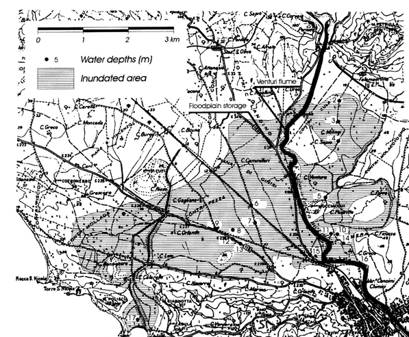
The study area is located in the southern part of Sicily and is crossed by the Imera river, one of the largest in the island with a basin of about 2000 km2. The main watercourse is about 150 km in length and it winds from the central part of the island to the Mediterranean Sea near to the city of Licata (Fig. 2). The alluvial areas are used intensively for agricul-ture activities with extended irrigation and many important transport facilities (railways, main roads, etc.). Residential areas and tourist accommodation are also established within the area at specific sites and the city of Licata (population 50 000) is located at the mouth of the river.
Fig. 2. Inundated area.
35
2
G.
Aronica
et
channel, to a coastal area. Unfortunately, only a part of the project was actually realized. A venturi flume was built in the before mentioned river section, in order to increase the water depth and to divert the excess flow through a side channel spillway placed in one side of the venturi flume. A small floodplain storage facility was constructed, close to the venturi flume, but no connecting artificial channel was made.
On October 12th 1991 heavy rainfall occurred over the whole Imera river watershed and caused one of the most severe inundations of the Licata plain in this century. The heavy rainfall started at 6.00am 12/10/91 and stopped at 12.00pm 12/10/91 with a total duration of 21 h, the total rain depth was 229 mm and the maximum intensity was 56 mm h¹1 with a total rain volume of 225 million cubic meters. The flow overcame the river capacity in the venturi flume and over-topped the flood banks in other sections, before passing through the city of Licata, without any significant urban flooding. However, the flood wave spread from the floodplain storage on the right hand side of the river, reaching a coastal area causing severe damage (Fig. 2).
The data available from this event for the model calibra-tion can be summarized as follows1:
1. The inundated area was delimited with a field survey carried out a few days after the event, the collected data was completed by analysing the requests for damage reimbursements submitted by the farmers to the government. The boundary of the inundated area is reported in Fig. 2.
2. During the same survey the trace of the maximum water level was observed and measured at 17 loca-tions points, such as on piers or concrete walls. This data is shown in Table 1. Further, maximum water levels observed in a river cross-section near the city and in an artificial channel near the bay, allowed the estimation of outlet peak discharges and time to peak in the bay (Table 2).
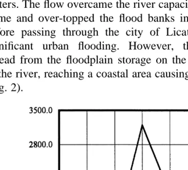
3. Because the upstream gauge was washed away during the flooding, the volume and the shape of the input flood hydrograph (Fig. 3) was obtained by a kine-matic rainfall/runoff model using rainfall data from several raingauges in the watershed area.
3.2 The finite element model domain
The limits of the finite element mesh were based upon the basin morphology in order to cover the inundated surface and to leave the upper areas out of the domain. The total domain area is about 22 km2, discretized in 3154 triangular elements. The geometric features (x,y,z coordinates) of the 1690 nodes were defined by digitizing contours from 1:2000 technical maps. The specific criteria in order to select the mesh nodes were cast hierarchically as follows: (1) points with known elevation; (2) points in areas with steep slope, approximated with vertical discontinuities, including the contour of the venturi flume and the flood-plain storage; (3) distinctive points for describing geometrical patterns of the river bed; and (4) distinctive nodes for describing geometrical patterns of the ground morphology.
The mesh was created from these nodes by using the GIS contouring package TIN that builds triangular irregular net-works from point data15. The final mesh is shown in Fig. 4.
4 CALIBRATION
To calibrate the unknown values of the model parameters, we want to find those which give simulated outputs (water level or flows) as close as possible to the observed data. Traditionally calibration of distributed model parameters Table 1. Survey data
Sites Measured water depths (m)
1 10.50
2 0.30
3 0.40
4 0.20
5 3.90
6 0.60
7 0.80
8 0.40
9 1.70
10 1.70
11 2.20
13 0.10
14 0.50
15 1.30
16 6.50
17 1.60
Table 2. Survey data
Sites Estimations
Qp-river 1700 m3s¹141900 m3s¹1
Qp-bay 500 m3s¹14600 m3s¹1
tp-bay h24.004h01.00
has involved minimizing the ‘error’ between the observation and the prediction. This error arises from differences between the model structure and the system being modelled and from the uncertainties in the available information.
The error can be measured using different forms of objective functions, based on a numerical computation of the difference between the model output and the observations.
In the traditional approach the purpose of calibration is ‘to find those values (an optimum parameter set) of the model parameters that optimize the numerical value of the objective function’23. Given that flood models are highly non-linear, we can expect to obtain the same or very similar values of the objective function for different parameter sets (non-uniqueness of the solution of the inverse problem), or different inflow series (for different flood events) can give a different goodness of fit for the same parameter sets. In this case, the idea that for a given model structure, there is some optimum parameter set that can be used to simulate the system loses credibility. There is rather an equifinality of parameter sets, where different parameter sets and therefore model structures might provide equally acceptable simula-tors of the system. This then leads to uncertainty in the calibration problem (parameter uncertainty) and related uncertainty in the model predictions8.
The GLUE procedure9, transforms the problem of searching for an optimum parameter set into a search for the sets of parameter values, which would give reliable simulations for a wide range of model inputs. Following this approach there is no requirement to minimize (or maxi-mize) any objective function, but, information about the performance of different parameter sets can be derived from some index of goodness-of-fit (likelihood measure).
In the proposed model the Manning’s roughness coefficient in eqn (2) is the unique parameter involved in the calibration. The model structure allows one coefficient for each triangular element to be used, but, lacking a good basis for allowing the roughness coefficient to vary, the flow domain was divided into 2 principal regions, over bank flow and river flow, and for both of these an ensemble average roughness coefficient was assumed. As a first approxima-tion, it is assumed that the effect of the inhomogeneities in the floodplain roughness on the flood wave becomes smoothed out and the overall response to a ‘lumped’ flood-plain roughness is examined in this paper. This reduced the dimensionality of the distributed parameter space from 3154 to just two for the calibration problem at this initial stage of characterizing the overall finite element model response. The roughness coefficients for these two regions were varied between two limits (see Section 5), and the goodness of fit was assessed using different objective functions. 1000 Monte Carlo runs of the flood model with different combi-nations of these two parameters were made on the Paramid parallel processing facility at Lancaster University, each simulation taking approximately two and a quarter hours on a single processor.
4.1 Calibration based upon statistical framework
For the type of complex distributed model considered here, observation errors and model structural errors will always exist, arising from a variety of indeterminate factors, so it is helpful to consider the inverse problem in a statistical framework. Unfortunately, there was no information regarding the uncertainties in the observations of water surface heights and these are taken to be absolute values, although the treatment of such an error is discussed in section 5.4.
4.1.1 Normal and heteroscedastic likelihood functions
The errors between the observed and predicted variables have the form:
«i¼yi,obs¹yi,
,(i¼1, …,r) (13)
where yi,obs denotes the observed variables at ith site and
yi,simdenotes the simulated variables at the same site. The
residual «i could be assumed to be white Gaussian and,
hence, its likelihood function would consist of r multiplica-tions of the conditional probability function for each observation of the residual «i:
Normal Gaussian joint probability:
where«iis the model residual at i-th site,jiis the variance
of the residuals at the i-th site and r is the number of data points.
Using eqn (14) is equivalent to making the following Fig. 4. Finite element mesh.
two assumptions concerning the probability distribution of the errors23:
1. The joint probability of the errors over the available data record is Gaussian with mean zero,
2. The errors are independent of each other with constant variance.
Very often data may violate these assumptions11and the effects can be non-trivial. Sorooshian and Dracup22 devel-oped maximum likelihood based objective functions to properly account for the presence of either autocorrelation (non-independence) or hetroscedasticity (changing var-iance) of data errors. Assuming uncorrelated errors, which may be appropriate in this case since the measurement sites are generally well separated, the form of the maximum like-lihood criteria was called HMLE (heteroscedastic maximum likelihood estimator) and has the form:
HMLE(v)¼
where:wi is the weight assigned to site i, computed as
wi¼h
2(l¹1)
i,obs andlis an unknown parameter linked to the
variances.
The HMLE estimator is the maximum likelihood, mini-mum variance, asymptotically unbiased estimator when the errors in the output data are Gaussian, uncorrelated with zero mean and have variance related to the magnitude of the output.
4.1.2 Application of the statistical error model to the calibration problem
Using the statistical framework, the different premises were based only upon the residuals of the water surface height predicted at 17 sites where observations were available. In eqn (14) and eqn (15) the residuals could alternatively be derived from differences between observed and predicted discharges or time to peak.
However, the ambiguity and scarcity of the information does not permit the analysis of the statistical properties of this alternative field data.
4.2 Calibration based upon fuzzy rules
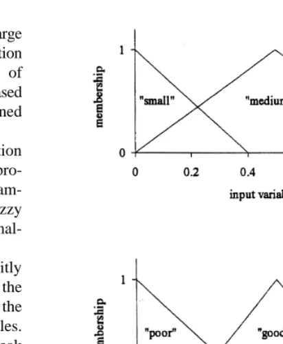
The use of fuzzy logic to construct a set of ‘‘if/then’’ rules is most suited to situations where there is very little informa-tion and where available informainforma-tion is highly ambiguous, such as the case in this study. A rule might be of the form: if the modelled flow is ‘well predicted’ on the basis of one objective function (the premise of a rule) then there is a ‘strong’ possibility that the model structure is relatively good (the consequent of a rule). The fuzziness in these qualitative terms can be represented geometrically in the
form of a membership function which allows for different degrees of membership of a set, e.g. the set of ‘well predicted’ flows.
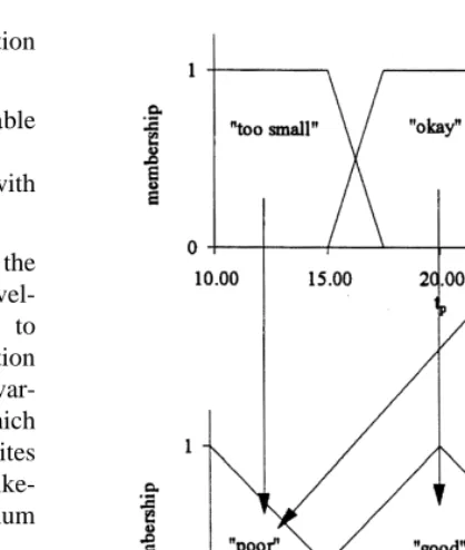
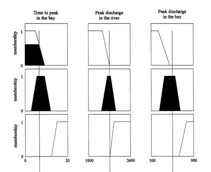
Fig. 5 shows how the universe of predicted times to peak discharge of the flood in the Imera Basin at a certain site can be divided into membership functions expressing our knowledge of the system in terms of fuzzy sets.
The arrows represent the three rules:
1. If predicted time to peak in bay is ‘too small’ then likelihood measure is ‘poor’
2. If predicted time to peak in bay is ‘OK’ then like-lihood measure is ‘good’
3. If predicted time to peak in bay is ‘too large’ then likelihood measure is ‘poor’
The premises in the sketch were chosen since they repre-sent one of the most ambiguous sets of information which were used in the calibration of the flood model. The shapes of the individual membership functions were chosen to be trapezoidal, since the flat top represents a lack of informa-tion regarding the true time to peak in the bay.
For the case before, there is only one premise for each rule, but more generally there are multiple premises which must be combined, as described in the next section.
4.2.1 Fuzzy sets
The formal definition of a fuzzy set4 is given here for example of the different predicted times of arrival of the peak flow in the bay
Let T be the set (universe) of predicted times of arrival of the peak flow in the bay. let TOKbe a subset of ‘OK’ times to
peak flow in the bay (i.e. the subset of predicted times to the peak discharge in the bay which roughly agree with the
observations). TOKis called a fuzzy subset of T, if TOKis a
set of ordered pairs:
TOK¼{(t,mTOK(t)); t[T,mTOK(t)[[0,1] (16)
wheremTOK is the grade of membership of t, the predicted
time of arrival of peak flow in the bay, in TOKand is termed
the membership function of TOK. A membership of 0 or 1
implies t absolutely does not or does belong to TOK,
respec-tively. Those membership grades between imply that t has partial membership of TOK. Three fuzzy subsets of ‘T’ are
used to describe the complete set of predicted times in Fig. 5, given by ‘too early’, ‘OK’ and ‘too late’, each having trapezoidal membership functions. The fuzzy sets of times of arrival of the peak discharges used here are special cases of the general description of a fuzzy set given by eqn (16), called fuzzy numbers. A fuzzy number satisfies the requirements:
1) For at least one value of t,mT(t)¼1
2) For all real numbers a, b, c with a, b, c:
mT(c)$min(mT(a),mT(b))
(the convexity assumption) (17) wheremTrefers to the membership function of an arbitrary
fuzzy subset of T. In this study triangular and trapezoidal shaped membership functions are used as shown in Fig. 5, which can both satisfy the before requirements4.
The support of a fuzzy number (for example the subset of ‘OK’ times of arrival of the peak discharge in the bay) is the range of values for which the membership function is non-zero, or formally:
supp(TOK)¼{t,mTOK(t).0: (18)
The general form of a fuzzy rule consists of a set of pre-mises, Ai,fin the form of fuzzy numbers with membership functions mAi,f, and a consequence Li (in this study the consequent will always refer to a likelihood measure), also in the form of a fuzzy number:
If Ai,1#Ai,2#……#Ai,f then Li (19)
where i refers to the rule number, and f to the piece of information the relation pertains to, for example in eqn (19), rule number 1, A1,2 might refer to the premise: ‘the
predicted time to peak discharge is OK’. The operator #
is the fuzzy logic equivalent of the Boolean logic ‘and’ or ‘or’ statement which is used to combine premises based on different pieces of information. The above rule might read Fig. 6. Schematic fuzzy inference system (based on Matlab fuzzy toolbox) showing fuzzy implication and fuzzy aggregation techniques
(see text, section 4.2).
‘if the predicted time to peak in the bay is OK and predicted peak discharge is OK then the likelihood measure is strong’.
There are several possible fuzzy logic equivalents of ‘and’ or ‘or’, although Bardossy and Duckstein4 report that there appears to be no great difference in the perfor-mance of the rule systems with respect to the choice of operator. Operators based on the product techniques were used here, since these maintain information from every pre-mise (so long as there is non-zero membership), whereas other techniques (min and max) work on the extreme values. The degree of fulfilment, viof each rule, i, is a measure of how well the rule is satisfied overall and is used to implicate the membership grade (indicated by the shaded regions in Fig. 6) in the consequent likelihood fuzzy number. The degree of fulfilment for the simple, one premise rule ‘if predicted time to peak discharge is OK then likelihood is strong’, is simply the membership grade of the predicted time to peak discharge in the fuzzy subset of ‘OK’ times to peak. The degree of fulfilment for a multi-premise rule depends on the choice of operator e.g. fuzzy logic equiva-lents of and can be the minimum or the product of the different membership grades for a particular vector of pre-mises (Ai,1…, Ai,f). Here ‘product inference’ based rules are used to determine the degree of fulfilment corresponding to ‘‘and’’ (uAi in eqn (20)) and ‘‘or’’ (uOi in eqn (21)):
uAi(Ai,1 and Ai,2…and Ai,3)¼
YF
f¼1
mAi,f(af) (20)
where F is the total number of pieces of information, afare the arguments to which the rules are to be applied. As an example we refer to the rule based on two pieces of infor-mation: ‘if the predicted time to peak in the bay is OK and predicted peak discharge is OK then the likelihood measure is large’. a1is the predicted time to peak discharge, a2is the
predicted peak discharge in the bay. The membership grades of these predictions in the fuzzy sets ‘OK times to peak’ and ‘OK discharges’ are:mAi,1(a1)andmAi,2(a2). The
degree of fulfilment of the rule overall is then the product of these two quantities.
For the probabilistic or statement, eqn (21) are used recur-sively for F pieces of information (for the example before there are only 2 pieces of information, so the first expression need only be evaluated):
The degree of fulfilment is then used to shape the conse-quent fuzzy number, Li, usually by truncating the member-ship function somehow. In this study a product type approach is used, where the degree of fulfilment is used to multiply the height of the apex of the triangular likelihood fuzzy number. The resulting ‘altered’ fuzzy numbers in the
consequent (likelihood measure) universe are shown schematically in Fig. 6, where it can be seen that they are generally overlapping. In the regions of overlap, different rules can influence the same part of the consequent universe, so a method of combination is once again required. This is achieved through the use of eqn (21) again, which represents a fuzzy union operation.
Finally, the resulting likelihood fuzzy numbers are defuz-zified by finding the centroid, C(L), which becomes the crisp output of the system, which in our case is a possibility measure for a particular parameter set21:
C(L)¼
where l is the likelihood measure or x-axis in Fig. 5. The crisp values, C(L), then define the likelihood surface in the parameter space.
4.2.2 Selection of the membership functions
The support of a membership function would normally be assigned based upon a set of training data comprising inputs and outputs, for instance see Bardossy et al.3. The universes of the premise and the consequent variables are typically divided up into a number of classes and assigned a linguistic description, such as a ‘small’ flow depth of water at each site. The number of classes we choose will depend upon the amount of information represented by the data, if we have very little data, then only a few classes are used. In this study, by reducing the continuum of modelled flow depths at any particular site into three sets, we can then incorporate our limited number of fuzzy observations. However, for the calibration problem, there is initially no ‘sample’ informa-tion concerning how the likelihoods (relative possibility measures) should be distributed. Therefore, we have to interpret the relationships between modelled and observed flows in terms of their partial memberships in fuzzy sets corresponding to poor, good and strong likelihoods. The support assigned to, for example a ‘strong’ likelihood, is chosen in order to correspond with our perception of how accurate the flow prediction needs to be in order that the model can be said to be a good predictor of the system, to within the uncertainties (fuzziness).
The amount of overlap of the fuzzy sets strongly influ-ences the shape of the resulting likelihood surface and for the case where there is no overlap, the surface becomes more unrealistically ‘stepped’. Clearly the choice of overlap is subjective in this study, although it was suggested that a good empirical rule is to allow 25% overlap17. The sensi-tivity of the likelihood surface to a parameter which varied the amount of overlap for one of the fuzzy sets is discussed in later sections.
4.2.3 Application of fuzzy sets to the calibration problem
where observations were available, the time to peak discharge in the bay, the peak discharge in the bay and at an observation point in the river (this making a total of 20 pieces of information). This illustrates the flexibility of the rule-based system, as different sources of information can be combined in the derivation of the consequent likelihood measure.
The information about the discharges and the information about the water surface height residuals were used to pro-duce two independent sets of fuzzy rules, which were exam-ined independently and in combination, by taking the fuzzy product (fuzzy logical ‘‘and’’ statement) of the re-normal-ized likelihoods (see figures later).
The different sources of information were not explicitly weighted, but, rather the relative degrees of fuzziness in the different sources were designed to be accounted for in the construction of the membership functions and fuzzy rules. For example, the fuzzy information about time to peak discharge was deemed less important than the fuzzy infor-mation about the water surface height, so the rules were constructed such that there was no premise based on the time to peak which results in a ‘strong’ possibility measure (whereas a ‘very small’ water surface height residual does lead to a ‘strong’ possibility measure).
Clearly a conditional statement in the form of eqn (19) which links together all 20 pieces of information available about the flood, using the fuzzy logic equivalent of ‘‘and’’ is highly stringent and would most likely result in very few cases where the likelihood had a high membership of the set of relatively ‘strong’ likelihoods. Conversely, a statement in the form of eqn (19) based upon the fuzzy logical equivalent of ‘‘or’’ tends to be too lenient a condition. For this method of combination, we can have the condition that if there is a single relatively small residual then, depending on the degree of membership of this residual in the fuzzy set of ‘small’ residuals, the overall likelihood measure will be relatively ‘strong’. The two extremes (‘and’ and ‘or’ com-bination) can be combined using a weight, g, such that the degree of leniency can be varied4 to provide an overall degree of fulfilment, Di, as in eqn (23):
Di¼g3ui(Ai,1or…orAi,f)þ
þ(1¹g)3ui(Ai,1 and…and Ai,f): (23) In this study a similar weighting function, G, is used after the aggregation and defuzzification stages such that the weighted sum of the two crisp outputs of the extremal cases becomes the overall output:
C(L)¼G3CO(L)þ(1¹G)3CA(L) (24)
where COand CAare the centroid of the consequent fuzzy set when fuzzy equivalents of ‘or’ and ‘and’ are used, respectfully. The two techniques before will essentially have the same effect, although the resulting crisp outputs will be slightly different because of the non-linear operations involved in the aggregation and defuzzification techniques. The possibility surface generated using different values of G is examined in section 5.2 later.
The first three fuzzy sets for the time of arrival of the peak flood at the bay, and the discharges at the bay and the river sites were of similar form to those in Fig. 5. These rules are represented schematically in Fig. 6, where the implication, aggregation and defuzzification processes are represented and were constructed using the Matlab fuzzy toolbox13.
The residuals of the maximum water surface height at each of the 17 sites (at which measurements had been made) were determined and compared against similarly constructed fuzzy sets, only one of which is shown in Fig. 7 for conciseness.
4.2.4 Sensitivity analysis of variable parameters in fuzzy system
Two variable parameters at the calibration stage were used to demonstrate the sensitivity of the resulting likelihood surfaces to changes in fuzzy-rule-based system construc-tion. The first, G, has already been introduced as a factor which exerts influence on the stringency or leniency of the rules. The other parameter, Sa, is the extent of the support for the membership function of a ‘small’ residual in Fig. 7. If Sais relatively small then there will be a tight criterion for residuals which have a high membership in the fuzzy set of ‘small’ residuals. Consequently, there will be a smaller membership of model predictions which are ‘strongly’ likely.
Equal intervals for the supports of the membership functions for residuals at each site were used in this study, although separate rules could be defined for each site which incorporated varying supports which could then account for heteroscedasticity in the residuals.
Fig. 7. Membership functions for sample input (water surface
depth residual) and output (likelihood measure) to a fuzzy rule.
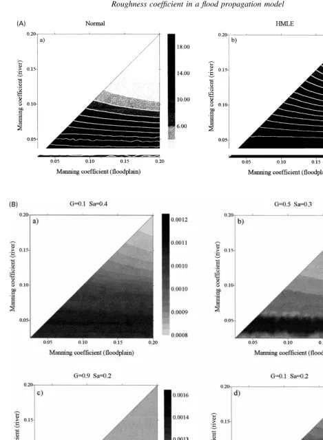
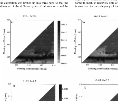
Fig. 8. (A) Likelihood measures for statistical calibration: water depth information only. (B) Likelihood measures for fuzzy-rule-based
calibration: water depth information only. Sais the support (defined in eqn (18)) of the fuzzy subset ‘‘small’’ residuals. G is the parameter
5 THE GLUE PROCEDURE
The GLUE procedure9 comprises several steps between generation of the likelihood surface over the parameter space and producing estimates of uncertainties in the pre-dicted model responses. These steps are outlined in the next few sections, in which those figures associated with the statistical calibration and the fuzzy-rule-based calibration are labelled (A) and (B) respectively.
5.1 Selection of the parameter ranges
The first step of the GLUE procedure is to decide upon the range of the parameter space to be examined, which relies upon ‘expert knowledge’ of the system. The two physical parameters to be calibrated in this study are the Manning coefficients, one to represent the roughness of the flood plain region and the other to represent the river bed. Clearly,
such a simple model structure does not reflect the true distributed roughness in the basin, and it becomes less imperative to find an optimum fit, as discussed earlier.
However, the initial decision as to the range of parameter space to be examined can exert an influence on the decisions to be made later, on the basis of the predicted uncertainties. For instance, having generated uncertainty bounds for the model predictions on the basis of a truncated range of rough-ness coefficients, caution must be taken when using these to disregard certain outlying predictions or to disregard obser-vations (the modeller might wish to use a truncated range of parameter values in order to assert some a priori knowledge about the physical situation in the field). It is considered that this problem can be largely overcome by initially using ranges of parameters which cover the extremes of feasible values, for example, in this study, Manning coefficients corresponding to bare soil, all the way to values correspond-ing to a highly rough floodplain were used10. This resulted
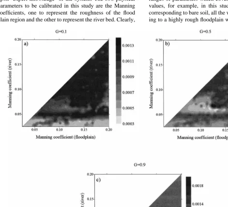
Fig. 9. (B) Likelihood measures for fuzzy-rule-based calibration, user discharge information only. G is the stringency parameter defined in
eqn (24).
in a range of roughness coefficients for c of 0.025 m¹1/3s¹1 and 0.2 m¹1/3s¹1to be used, with the restriction that the roughness of the river could not exceed the roughness of the floodplain, hence, the triangular parameter domain on the possibility measure plots. Bates et al.7 used Manning values for the channel ranging between nc¼0.01 m
¹1/3
s¹1
(corresponds to a concrete lined channel) to
nc¼0:05m
¹1=3
s¹1 (corresponds to a mountainous
stream with a rocky bed) and for the floodplain, they used
nf ¼ 3ncþ 0.01. The 1000 different combinations of the
Manning coefficients within the triangular domain described before were used to generate the likelihoods or relative possibility measures.
5.2 Generation of likelihood surfaces
The calibration was broken up into three parts so that the influences of the different types of information could be
examined more closely. Fig. 8 shows the likelihood measures over the parameter space for the case where only the water surface height information is used. Fig. 9(B) shows the likelihood surface for the case where only the information about the peak discharges was used and finally Fig. 10(B) shows the likelihood surface were all the 20 pieces of information are used.
For the fuzzy calibration, the sub-plots in each case demonstrate the effect of varying the two calibration para-meters discussed before. The variation of the support size Sa was included to demonstrate how its choice can influence the overall output. Normally it would be selected at an intermediate value, based on experience, which allowed a reasonable number of parameter combinations to influence the resulting surface. It can be seen that for small Saand large G, the condition for a strong possibility measure is harder to meet, so relatively little of the possibility surface is sensitive. As the stringency of the rules is increased, so
Fig. 10. (B) Likelihood measures for fuzzy-rule-based calibration: combined information. Sais the support (defined in eqn (18)) of the
the technique becomes more similar to an optimization process.
From inspection of the different figures, for all the differ-ent combinations of G and Sa, it becomes clear that the roughness values for the river with the greater likelihood measures are in the approximate range c¼0.04 m¹1/3s¹1to 0.06 m¹1/3s¹1. Since the ‘ridge’ of relatively more possible parameter combinations exhibits an insensitivity to the floodplain roughness for most of the likelihood surfaces, then we should conclude that there is insufficient data with which to constrain the current model in order to gain more information about the floodplain roughness.
However, inspecting more closely the lower right sub-plot of Fig. 10(B), which utilizes all of the calibration information and represents the most stringent set of fuzzy rules, the truncated ridge of more possible floodplain rough-ness values (c ¼0.025 m¹1/3s¹1¹0.12 m¹1/3s¹1) can be interpreted as representing the region of more feasible Manning coefficients. Such results however need careful interpretations. The fact that we have used the stringent fuzzy calibration requires that in order for the likelihood measure to be strong, all of the residuals for the water surface heights must be independently small and the predic-tions concerning the discharges be all independently good. In making this assertion, we are relying on these pieces of information to be independent. If we wish to make conclu-sions about the approximate ranges of more acceptable manning coefficients for the two regions, then our conclu-sions should therefore be ‘On the basis of the Monte Carlo analysis, the floodplain roughness was constrained to lie within the approximate range (c ¼ 0.025 m¹1/3s¹1 ¹
0.12 m¹1/3s¹1) and that the river roughness can be approximately constrained to lie within the range (c ¼
0.04 m¹1/3s¹1to 0.06 m¹1/3s¹1)’. Earlier in the study we assumed independence in the residuals, on the basis that the measurement sites corresponded to regions within the flow domain which were spatially far apart. If we discover new information which contradicts our assumption then we must consider that the set of rules which were used in order to produce the constrained range of Manning coefficients, represent an over-constrained system.
5.3 Generation of cumulative likelihood plots
The next stage of the GLUE procedure is to arrange the residuals or other predicted observables into ascending order and to plot the cumulative likelihoods determined before against the size of the predicted observable (Fig. 11). Considering the water surface height residuals only, (for which the information available is less fuzzy) it is apparent that at one of the sites, in the river, the water surface is highly sensitive to the roughness coefficients. In case these large variations were caused by unusual parameter
Fig. 11. (A) Cumulative likelihood of 17 predicted depths using
the statistical calibration. (B). Cumulative likelihood of predicted depths at 17 sites using the fuzzy calibration (G¼0.5, Sa¼0.3).
combinations, an analysis was made whereby the parameter pairs which gave rise to predicted water surface height residuals greater than 1 m were excluded. However, this resulted in over half of the parameter pairs being excluded, many of which were predicting sensible residuals else-where. For this reason the sensitivity was put down to a more physically intuitive explanation: the roughness coeffi-cients determine whether or not a large volume of water will be directed through the relatively narrow river channel, so the water surface height at this point was bound to be sensitive to the roughness parameters.
Conversely, there are some sites at which the water surface height is highly insensitive to the roughness coefficients, which correspond to locations on the extensive flat regions of the basin, where damping would be expected.
At one site, there is apparently a double peak to the possibility measure, which results in a pronounced point of inflection on the cumulative plot. This demonstrates the importance of avoiding parameter optimization.
5.4 Generation of the uncertainty bounds on the predictions
Predicted observable pairs corresponding to the 10% and 90% percentiles limits of the cumulative distributions are used next to estimate uncertainties in the model predictions.
Predicted observables, which fall outside these limits, are generally considered, in relation to all the other predictions covering the feasible parameter space, as outlying points. This presents some contradictions for the cases such as that at site 7, where there are two ranges (there may be multiple ranges) of water surface heights which both apparently have fairly strong likelihood measures. For this reason, it is sug-gested that, before making any strong inferences based upon the uncertainty bounds, the distributions of the likelihood measures for all of the predicted depths are examined carefully.
It can be seen from the plots Fig. 12 that the water surface heights at sites 8, 12, 13 fall outside of the error bars (sites 8 and 12 are only just outside the error bars). It is possible that some of these deviations are caused by errors in the observed data, e.g. wave induced errors. Although there was apparently no wind at the time of the flood, the maximum tide mark at different sites will inevitably been affected by surface waves. There are also errors arising from the difference between the interpolated finite element mesh and the actual topology. These might be estimated to give uncertainties of approximately 5%– 10%. In the light of this information, the only problematic site is number 13.
Fig. 12. (A) 10 and 90% percentiles of model predictions using
the statistical calibration (observed data ‘o’). (B) 10 and 90% percentiles of model predictions using the fuzzy calibration
However, the possibility that the model structure is not an adequate representation of the flow processes must also be considered because of the poor fit at site 13, this will be investigated in future work by increasing the number of different regions having different roughness parameters, to reflect more accurately the heterogeneity of the true basin roughness. Similarly, the apparent failure to predict the cor-rect water surface height everywhere may were caused by an error in the modelled input hydrograph. Nonetheless, considering that once the uncertainties in the observations were taken into account, only the water surface height at site 13 is not within the 10% and 90% percentiles, the hugely simplified floodplain roughness parameterization was shown to be relatively flexible. Of course the approach requires additional data for further validation, since there are clearly relatively few observations available in this study.
6 FURTHER DISCUSSION
The possibility surfaces and the uncertainty plots produced by the various techniques are remarkably similar, which affords a degree of confidence in the techniques.
The possibility surfaces, which were obtained from the simple ‘if/then’ rules, appear to be equally, if not more useful than the measures obtained using the statistical error models, in the context of this study. The variation of the stringency parameters was found to be especially useful for visualizing the variation of the likelihood measure as they were varied from highly stringent (comparable to an optimization process) to less stringent (to allow a wider spread in the likelihood surface).
The uncertainty in the observations could in future be incorporated into the objective function, by formulating the observation as a fuzzy set and calculating the ‘fuzzy distance’4 between this and the fuzzy sets comprising different classifications of residuals.
With a more detailed set of observations, the information about correlations between measurement sites and the resulting correlations between error measurements could be included into the fuzzy framework. For instance, if the error measurements at two sites are strongly correlated, then there is a redundancy of total information, which can be gained from the two sites. The possibility measure could easily be made to reflect this by penalizing information from strongly correlated sources.
We aim to update the likelihood measures, as more information becomes available. This can be achieved in a Bayesian framework18 or an equivalent fuzzy updating technique, which is currently being tested.
7 CONCLUSIONS
The GLUE procedure was applied to a complex distributed model, on the basis of very little information, using two
different techniques, based around statistical error model and fuzzy-rule-based systems. Both techniques clearly incorporate judicious assumptions, whether it be inferences about the correlations in the distributed errors in the error model or the selection of support sizes for membership functions in the fuzzy model. However, this does not negate the usefulness of the two techniques, which if combined with expert knowledge of the system in hand and used sensibly to produce relative likelihood or possibility measures via the GLUE procedure, allow for a greater understanding of the model predictions. For instance, if there is equifinality (in terms of likelihood measures) of different model predictions to within the uncertainties in the measurements and model structure (as was found before with models of this type), then the GLUE procedure exposes this behaviour.
The fuzzy calibration therefore addresses the problem, which stems from attempting to fit a certain structure of physically based model on the basis of uncertain data. We argue that there will always be a degree of non-random uncertainty in our knowledge of systems as complex as the Imera basin, so the chimera of a precisely defined model structure will disappear each time we discover a new model structure which is equally acceptable on the basis of the data (the equifinality problem). It is accepted that the data set in use here is highly sparse and the model structure does require further improvements (more sub-domains having different roughness, etc.), but we have put forward the fuzzy calibration techniques as a general technique.
The statistical calibration technique, despite its advantages, e.g. it is easy to incorporate into both the statement of defining the inverse problem and into the GLUE procedure, is limited in this type of analysis where there is ambiguous initial data and limited observa-tions. For such scenarios, it is often difficult, if not impossible, to evaluate properly the statistical properties of the residuals.
On the contrary the fuzzy calibration technique, in so far as it was developed for use with the GLUE procedure, is useful on several accounts:
1. The rules are transparent and simple to implement; 2. Different sources of information and their relative
importance can be incorporated into the rules; 3. The decision-maker for the acceptability of a given
model structure can be assigned different degrees of ‘decisiveness’. The usefulness of this is best explained by example, take the case of a model based upon a sparse data set in which there are cor-relations present in the model structure (in higher dimension parameter space these become even more difficult to quantify) then a stringent optimization pro-cess could result in assigning too much precedence to information from sources which are essentially sup-plying the same information, leading to a falsely constrained system.
ACKNOWLEDGEMENTS
This work was supported by NERC grants GR3/8950 and GR3/10687. The authors would like to express their grati-tude for useful discussions about GLUE and other fuzzy procedures within the Environmental Science department at Lancaster and for computer support from K.Buckley.
REFERENCES
1. Aronica, G., Inondazione delle zone vallive dei corsi d’acqua: propagazione di un’onda di piena su superfici fortemente irregolari. Ph.D. thesis, Istituto di Idraulica, Universita` di Palermo, February 1996.
2. Aronica, G., Nasello, C. and Tucciarelli, L. A 2D multilevel model for flood wave propagation in flood affected areas. ASCE — J. Water Resour. Plann. Mgmt, 1998, 124(4), 210–217. 3. Bardossy, A., Bronstert, A. and Merz, B. 1-,2- and 3- dimen-sional modelling of water movement in the unsaturated soil matrix using a fuzzy approach. Adv. Wat. Resour., 1995,
18(4), 237–251.
4. Bardossy, A., Duckstein, L., Fuzzy rule based modelling applications to geophysical, biological and Engineering systems, CRC Press, Boca Raton, FL, 1995.
5. Bates, B. C. and Townley, L. R. Nonlinear discrete flood event models 1. Bayesian estimation of parameters. J. Hydrol., 1988, 99(1/2), 61–76.
6. Bates, P. D., Anderson, M. D. and Hervouet, J. M., Compu-tation of a flood event using a two-dimensional finite element model and its comparison to field data. In Modelling Flood Propagation Over Initially Dry Areas, ed. P. Molinaro and L. Natale. ASCE, New York, 1994.
7. Bates, P. D., Anderson, M. D., Price, D., Hardy, R. and Smith C., Analysis and development of hydraulic models for flood plain flow. In Flood plain Processes, ed. M. G. Anderson, D. E. Walling and P. D. Bates, Wiley, 1996.
8. Beven, K. J. Prophecy, reality and uncertainty in distributed hydrological modelling. Adv. Wat. Resour., 1993, 16, 41–51. 9. Beven, K. J. and Binley, A. The future of distributed models: model calibration and uncertainty prediction. Hydrol. Process., 1992, 6, 279–298.
10. Chow, V. T., Open Channel Hydraulics, McGraw-Hill, New York, 1959.
11. Clarke, R. T. A review of some mathematical models used in hydrology, with observations on their calibration and use. J. Hydrol., 1973, 19(1), 1–20.
12. Huyakorn, P. S. and Pinder, G. F., Computational Methods in Subsurface Flow, Academic Press, Orlando, 1983.
13. Jang, J. -S. R. and Gulley, N., Fuzzy Logic Toolbox for use with MATLAB, The Math Works Inc., 1995.
14. Jang, J. -S. R. ANFIS: Adaptive neuro-network based fuzzy inference systems. IEEE Trans. Systems, Man Cybernetics, 1993, 23(3), 665–668.
15. Kuniansky, E. L. and Lowther, R. A. Finite-element mesh generation from mappable features. Int. J. Geog. Inf. Systems, 1993, 7(5), 395–405.
16. Narasimhan, T. N. and Witherspoon, P. A. An integrated finite difference method for analysing fluid flow in porous media. Water Resour. Res., 1976, 12(1), 57–64.
17. Pesti, G., Shrestha, B. P. and Duckstein, L. A fuzzy rule-based approach to drought assessment. Water Resour. Res., 1996, 32(6), 1741–1747.
18. Romanowicz, R., Beven, K. J., and Tawn, J. A., Evaluation of predictive uncertainty in nonlinear hydrological models using a Bayesian approach. In Statistics For The Environ-ment 2: Water Related Issues, ed. Barnett and Turkman, Wiley, 1994.
19. Romanowicz, R. and Beven, K. J., Predictive uncertainty in distributed models: likelihood functions, the value of calibra-tion data and GIS visualisacalibra-tion techniques, CRES Technical Report TR/135, 1996.
20. Romanowicz, R., Beven, K. J. and Tawn, J., Bayesian calibration of flood inundation models. In Flood Plain Pro-cesses, ed. M. G. Anderson, D. E. Walling and P. D. Bates, Wiley, 1996.
21. Ross, T., Fuzzy Logic with Engineering Applications, McGraw-Hill, New York, 1995.
22. Sorooshian, S. and Dracup, J.A. Stochastic parameter estima-tion procedures for hydrologic rainfall-runoff models: correlated and heteroscedastic error cases. Water Resour. Res., 1980, 16(2), 430–442.
23. Sorooshian, S. and Gupta, V. K., Model calibration. In Computer Models of Watershed Hydrology, ed. V. P. Singh, Water Resources, 1995.
24. Tucciarelli, T., Aronica, G. and La Loggia, G. Studio della propagazione delle onde di piena su alveo inizialmente asciutto. Idrotecnica, 1995, 5, 299–307.