DERIVATION OF FOREST INVENTORY PARAMETERS FOR CARBON ESTIMATION
USING TERRESTRIAL LIDAR
Om Prakash Prasada, Dr. Yousif A. Hussinb, Michael J.C. Weirb, and Yogendra K. Karnac a Lecturer, Institute of Forestry, Tribhuwan University, Hetauda, Nepal - opkalwar540@gmail.com b
Department of Natural Resources, Faculty of Geo-information Science and Earth Observation (ITC), University of Twente, 7500 AE Enschede, The Netherlands - (y.a.hussin, m.c.weir)@utwente.nl
c Under Secretary (Tech.), President Chure-Tarai Madhesh Conservation Development Board, Government of Nepal, Khumaltar, Lalitpur, Nepal - karnayogendra@gmail.com
Commission VIII, WG VIII/7
KEY WORDS: Terrestrial LiDAR, Point Cloud Data, Tropical Rain Forest, Inventory Parameters, Above Ground Carbon Estimation
ABSTRACT:
This research was conducted to derive forest sample plot inventory parameters from terrestrial LiDAR (T-LiDAR) for estimating above ground biomass (AGB)/carbon stocks in primary tropical rain forest. Inventory parameters of all sampled trees within circular plots of 500 m2 were collected from field observations while T-LiDAR data were acquired through multiple scanning using Reigl VZ-400 scanner. Pre-processing and registration of multiple scans were done in RSCAN PRO software. Point cloud constructing individual sampled tree was extracted and tree inventory parameters (diameter at breast height-DBH and tree height) were measured manually. AGB/carbon stocks were estimated using Chave et al., (2005) allometric equation. An average 80% of sampled trees were detected from point cloud of the plots. The average of plots values of R2 and RMSE for manually measured DBHs were 0.95, 2.7 cm respectively. Similarly, the average of plots values of R2 and RMSE for manually measured trees heights were 0.77, 2.96 m respectively. The average value of AGB/carbon stocks estimated from field measurements and T-LiDAR manually derived DBHs and trees heights were 286 Mg ha-1 and 134 Mg ha-1; and 278 Mg ha-1 and 130 Mg ha-1 respectively. The R2 values for the estimated AGB and AGC were both 0.93 and corresponding RMSE values were 42.4 Mg ha-1 and 19.9 Mg ha-1 respectively. AGB and AGC were estimated with 14.8% accuracy.
1. INTRODUCTION
There is a growing need of accurate and effective methods for estimating forest biomass/carbon stocks to meet the requirements of both Kyoto Protocol and UN-REDD programmes (Castedo et al., 2012). The REDD+ Measurement, Reporting and Verification (MRV) requires accurate and precise estimates, a large number of reference plots must be established, which inevitably increases the time and effort and expense of the method.
The use of remote sensing techniques is critical for assessing fine-scale spatial variability of tropical forest biomass/carbon stock over broad spatial extents (Clark et al., 2011). Most exiting methods, which include indirect and direct measurement techniques, are limited in their capability to acquire accurate and spatially explicit measurements of forest tree-dimensional structural parameters.
The accuracy of ground-based forest inventory depends on many factors: the selection of locations to be surveyed, the number of points or plots to be surveyed, the skill level of individuals conducting the survey, type of equipment used, and data analysis methods. Apart from these, it also depends upon the forest canopy characteristics (for example, dense, sparse, open, closed or overlapping). Therefore, there is a need for the development of a new method for ground inventory that is more accurate, fast, reliable, more objective, less expensive, and operational than the conventional methods used to date.
T-LiDAR provides a noble solution for collecting reference data in any forest environment (Liang et al., 2012). T-LiDAR is one of the rapidly growing interests in photogrammetry as an efficient technology for fast and reliable characterization of 3D forest canopy via point cloud data acquisition (Tansey et al., 2009). The main advantages lie in its potential to improve the accuracy and efficiency of field inventories and to provide additional features for forestry applications.
Recent advances in T-LiDAR technology have made LiDAR data widely available to study vegetation structure characteristics and forest biomass. It may provide an alternative for the permanent sample plot method for ground-based forest inventory. T-LiDAR demonstrates promises for objective and consistent forest metric assessment, but further work is still needed to refine and develop automatic feature identification and data extraction techniques (Hopkinson et al., 2004).
2. STUDY AREA
The study area was located at the Belum State Park (RBSP), which is situated in the north of Perak State in Malaysia. The location of the study area in RBSP is shown in the Figure 1. The major land cover types of the study area were forest, and water. The majority of the forest species were characteristic of the tropical rainforest that in the Peninsular Malaysia. The main forests types belonged to the Dipterocarpaceae family which included tree species of Syzygium, Vatica, Mastixia trichotoma Blume, Pimelodendrom, Koompassia Malaccensis, Trypanosoma and others.
Figure 1. Map showing location of the study area (inset, location in Malaysia)
3. METHODS
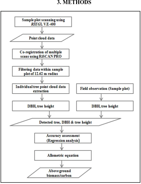
Figure 2. Flow diagram of research methods
The major three activities were carried out for conducting this research. They were field data collection, data analysis, and biomass and carbon estimation. In the field, both biometric data
and T-LiDAR point cloud data were collected. In biometric data, tree species, height, DBH, crown base height, crown diameter and plot crown density were recorded from direct observations. Point cloud data was collected using RiEGL VZ-400 T-LiDAR. RiSCAN PRO software was used for pre-processing, registration of multiple-scans, and manual measurement of tree parameters. Above ground biomass and carbon were estimated using allometric equation from both field observed and T-LiDAR derived DBH and tree height. Comparison among plots level inventory parameters, and AGB/carbon derived from T-LiDAR data and field measurements were done in RStudio. The research methodology is summarized in flow diagram of the research methods in Figure 2.
3.1. Plot delineation and T-LiDAR data acquisition
3.1.1. Plot establishment
After identification of plot, central scan positions were located such that there was minimum occlusion in the scanning. The trees very close to the plot centre, cause large area behind it to be in its shadow (Liang et al., 2012). The central positions were marked on the basis of ocular judgment. Since most of the plots were on sloping terrain, the central position was located such way that there was suitable and enough space for placing three outer scan positions. Some undergrowth in line of reflectors was cleared to get clear view from all four scan positions. Clearing also minimizes occlusion and gives a good scan of the bole of tree. All identified trees were marked with number tag as shown in Figure 3.
3.1.2. Placing reflectors
Twelve cylindrical and four circular reflectors were placed in each plot. All the plots were full of undergrowths, and therefore sticks were used to place cylindrical reflectors. Between each central and outer scan position four cylindrical reflectors were placed in such a way that they were visible from both position. The main purpose of using of cylindrical reflectors is to register the outer scan position to the centre scan position. Circular reflectors were placed randomly on marked tree stem facing towards centre scan position as shown in Figure 3. The circular reflectors were used for georeferencing of the plot.
Figure 1. A sample plot photograph showing arrangement of reflectors and tree tagging
3.1.3. T-LiDAR data acquisition
from surrounding vegetation as shown in Figure 4. In comparison to single scan mode, the multiple san mode give much more details of the scene but it takes more time for data acquisition and processing (Bienert et al., 2006). The scanning resolution of approximately 1 cm at a distance of 10 m was selected, because this is enough to distinguish small vegetation features like small branches and leaves (Feliciano et al., 2014). The following steps were followed to scan the sample plots.
Figure 4. Multiple scan mode (Bienert et al., 2006)
3.1.3.1. Fixing scan positions
At first central scan position was determined and from that point outer three scan positions were marked. Proper distribution of the 3 outer scans position with respect to the central position and circular plot was maintained in such a way that the angles between two out scans with the centre was around 120 degree (Figure 4). Tripod was placed on each scan position and the centre point was marked on the ground and GPS reading of the scan position was taken.
3.1.3.2. Setting T-LiDAR
After placing T-LiDAR on the tripod, camera was mounted on the top. Then level of the T-LiDAR was checked and legs of tripod were adjusted to minimize the roll and pitch of the TLS and instrument was set according to the technical specification given in Table 1.
Beam divergence 0.35 mrad Minimum range 1.6 m Pulse recetition
rate
300 kHz
Azimuth range 0°-360° (0.06° angular sampling) Zenith range 30°-130° (0.06° angular sampling) Acquisition time 1 min 23 s
Table 1. Riegl VZ-400 scanner settings for data acquisition
3.1.3.2. Fixing scan position and scanning
New project was set for each plot. Within the plot, each scan was saved as new scan-position. After that instrument was set for pulse ranging scan. Scanning was done at each position.
3.1.3.3. Fine scanning of reflectors
Fine scanning of reflectors is necessary for automatic registration of multiple-scans. For fine scanning, first automatic searching of reflectors were done. After that reflectors were identified and marked manually by locating on scanned data. Then fine scanning of marked reflectors were done automatically by setting the scanner in fine scanning mode.
3.2 Biometric data collection
Plot inventory data (DBH and tree height) of all trees within the sample plots were collected through direct observations. According to Brown, (2002), trees below 10 cm DBH contribute little to the total biomass of forest. Therefore, only trees having 10 cm or more DBH were measured. A diameter measuring tape was used to measure DBH of each tree at 1.3 m height above the ground. In addition, other important observations i.e. aspect, slope, and exposure were recorded. In the case of buttresses at 1.3 m, DBH was measured just at the end point of the buttresses. In the case of forked trees, if the fork was below the DBH, both trunks were measured as individual tree. The DBH reading was recorded up to millimetre accuracy so that it can be compared with T-LiDAR derived DBH. Laser range finder (Leica DISTO D5) was used to measured height of trees. The reading of height was recorded up to centimetre accuracy.
3.3. Manual extraction of inventory parameters
3.3.1. Pre-processing and multiple scans registration
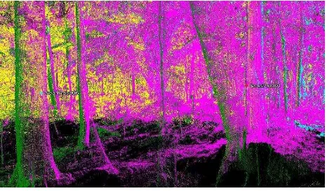
RiSCAN PRO v1.8.1 software was used for pre-processing of scanned point cloud data. The scanned file was imported as a new project using 'Download and Convert' wizard of help menu. All the three outer scan positions were registered to the central scan position using tie-points. The common tie-points between two scan positions were automatically identified by the program and were registered. An example of registered plot is shown in Figure 5. The scans from four positions have been displayed in fuchsia, yellow, aqua, and lime colour. The black colour is shadow area due to occlusion. To minimize the error in registration of multiple scans, 'Multi-Station Adjustment' was done. The error of multiple registration of plot varies from 11mm to 35 mm with an average of 16 mm for the 24 sample plots .
3.4. Manual extraction of individual tree
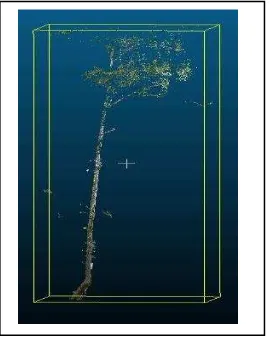
The registered point cloud data of sample plots were processed in RiSCAN PRO software for manual extraction of individual tree. Tree tag numbers were used to identify the individual tree. All point cloud representing the individual tree were separated from sample plot data using selection tool. The selection of all point cloud data associated with a single tree was performed by locating each marked individual tree stem within the entire plot point cloud and then selecting the vertical area corresponding to maximum crown diameter and tree height. In most cases the selected point cloud often included portions of canopy from surrounding trees. The individual tree point cloud data of all sample trees were visually inspected, and outlying point cloud were deleted. An example of extracted point cloud data of a tree was show in Figure 6. The manual extraction of individual trees was a time consuming task.
Figure 6. An example of extracted point cloud data of a tree
3.5. Manual measurement of DBH and tree height from T-LiDAR data
The Diameter at Breast Height (DBH) is defined as the diameter of the stem at 1.3 m above plane ground at base of a trunk. It was measured using distance measuring tool in RiSCAN PRO software. The tree height was measured in CloudCompare by box fitting in each tree as shown in the Figure 7.
Figure 7. Tree height measurement by box fitting in
CloudCompare software4. RESULT AND DISCUSSION
4.1 Tree species distribution
The forest of Royel Belum State Park is a protected primary forest having dominant species belonging to dipterocarpaceae family. Shorea, Hopea, Dipterocarpus and Vatica are the largest genera found in the study area. Biometric data was collected from 24 sample plots from area of 1.2 hectare of forest among which total of 59 tree species were recorded. Around 62% of forest area is covered by seven major species, among them 15% by Syzygium species, 13% by Vatica species, 9% by Mastixia trichotoma Blume, 7% by syn. Acacia greggii, 7% Pimelodendrom species, 7% by Koompassia Malaccensis and 6% Trypanosoma species. The details of forest species distribution are shown in Figure 8.
Figure 8. Species distribution in the study area
4.2 Tree detection and accuracy assessment
To assess the accuracy of trees detected from point cloud data, manually detected trees per plot were compared with respect to field observations. The tree extraction percentage in plots were varied from 69 to 100 as shown in Figure 9.An average 89 % of the field observed trees were detected from the point cloud data. In the plots 2, 7, 9, 12, and 14 all the sample trees were identified and detected, while in other plots less number of trees detected. The main causes of lower tree detection rate in other plots were occlusion (Figure 12) due to high stem density and the presence of undergrowth. Some tags were not identified due to occlusion. These results are similar to the results of Othmani et al., (2011). They got an average detection rate of 90.6% with single scan using the Computree algorithm.
Figure 9. Manual detection rate of trees per plot 0
20 40 60 80 100
1 3 5 7 9 11 13 15 17 19 21 23
De
te
ctio
n
r
a
te
(%
)
Plots Manual detection of plot
4.2 DBH measurements and accuracy
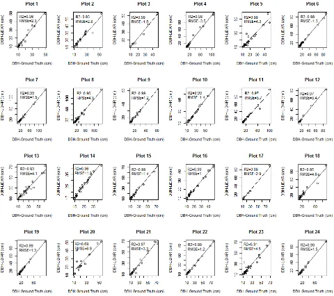
Regression analysis was done to compare the relationship between field observation and T-LiDAR derived DBH. The scattered plots are shown in Figure 10.
The lowest value of R2 was 0.69 in plot 27 and the highest value was 0.99 in plots 6, 7, 9, 10, 16, 17, 20, 24, and 26. The plots 5, 21, and 25 have outliers which had decreased the overall value of the plots. These outliers were due to occlusion (Figure 14) due to high stem density and undergrowths.
The average value of R2 of all plots was 0.95, which is very high reasonable estimate for the manual measurement of tree DBH from 3D point cloud data with an average RMSE value of 2.7 cm.
Several studies have similar results which support the findings the this study. Hopkinson et al., (2004) found R2 value 0.85 and regression slope value 1.01 for DBH in deciduous forest. In a similar study conducted by Tansey et al., (2009), RMSE values
between 1.9-3.7 cm was found. In a study conducted by Kankare et al., (2013) in Scots pine and Norway spruce stands, R2 value 0.95 and RMSE value 1.48 cm were obtained by manual measurement. Similarly, Maas et al., (2008) obtained RMSE value 1.8 cm for DBH measurement in inventory plots from Spruce and Beech forests. According to them T-LiDAR has limitations to use in natural forest having dense undergrowths in comparison to plantation forest with less complex structure and sparse ground vegetations. Tansey et al., (2009), reported a similar figure for RMSE values of 3.7 and 1.9 cm computed by cylinder-fitting and circle-fitting. Watt & Donoghue, (2005), found R2 value 0.92 by circle fitting in conifer plantation forest.
Thus, the values of R2 and RMSE for DBH measurements by manual methods from T-LiDAR data are consistent with many previous studies conducted in temperate forest, which shows that DBH can be estimated from point cloud data with good accuracy in tropical forest too.
4.3 Tree height measurements and accuracy
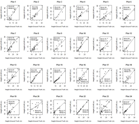
Regression analysis was done to compare the relationship between field observed and manually measured tree heights from T-LiDAR data. The scattered plots are shown in Figure 11.
The lowest value of R2 is 0.38 for plot 5 and the highest values is 0.99 for plot 22. The plots 3, 14, 15, 22 and 24 have R2 values higher than 0.90, while other plots have lower values due outliers. The average value of R2 of all plots is 0.77, which is a reasonable estimate for the manual extraction of tree height from 3D point cloud data for AGB and AGC estimation with an average RMSE value of 2.96 m.
In this study average manual measurement of tree height was overestimated by approximately 8% in compared to the field measurement. But in a similarly study by Hopkinson et al., (2004), they found R2 value 0.86, and regression slope 1.08 for deciduous forest. In their study, the tree height was underestimated by 7% in comparison of field measured height. According to them intervening foliage obstructing the view which leads to leads to systematic under estimation of tree
height derived by T-LiDAR. Thus, this study contradicts with the finding of Hopkinson et al., (2004), and shows that tree height can be measured more accurately in comparison to field measurement.
The main causes of outliers are occlusion and overlapping crown in upper canopy of the trees (Figure 14). Due to overlapping crown, in many cases it was impossible to separate whole crown of a tree, particularly for the small tree. Therefore, in manual extraction of individual tree from sample plot point cloud data, prior information about crown size is required for dense crown cover class forest. Thus, manual measurement of tree height from the T-LiDAR data is as subjective as manual tree height measurement in the field.
In the tropical forest generally trees have big crown size which makes difficulties in locating actual peak of the tree. This phenomenon leads to underestimation of large tree. The reason for the improvement in the height measurement is may be due to the improvement in capacity of T-LiDAR or may be human error. Therefore, further research is necessary to test the accuracy of tree height measurement using T-LiDAR data.
4.5 Above ground biomass and carbon stocks
AGB of the sample plots were estimated using the allometric equation of Chave et al., (2005). Conversion factor 0.47 was used to convert AGB to Carbon stock (IPCC, 2006). The details of ABC stocks in the sample plots are given in Figure 12. The AGC stocks in the plots 4, 7, and 8 are overestimated while in plot 6, the values is equal, and the rest of the plots are underestimated in comparison with field estimation. The main reason for overestimation is the difference in height measurements. The lowest stock of AGC is 37 Mg ha-1 in plot 1 and the highest is 361 Mg ha-1 in plot 4. The average per hectare estimate of carbon are 134 Mg from field observation and 130 Mg on the basis of T-LiDAR estimation. The average AGC stock was under estimated by 3% from T-LiDAR in comparison of field estimate.
Figure 12. Plot comparison of AGC stocks
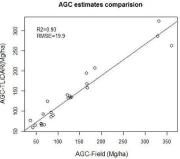
Figure 13. Comparison of AGC stocks
In the scattered plot (Figure 13), the R2 value of the estimated AGC stock is 0.93 and the corresponding RMSE value is19.9 Mg per hectare. Per hectare RMSE% value for AGC is 14.8%. The three plots in the top have big diameter trees which make big difference in AGC stocks with respect to other plots. The R2 value show that AGC can be accurately estimated with T-Scots pine and Norway spruce forest, R2 values were 0.90 and
0.91 and RMSE values were 22.12 kg and 26 kg achieved at tree height measurement both in field (specially tree height) and T-LiDAR measurement. Manual DBH measurement from T-LiDAR data are affected by stem form (Kankare et al., 2013). This variation is due to noncircular shape of the trunk. The reading of two perpendicular diameters are not equal. In this study only one diameter reading at 1.3 was measured. Other sources of errors were shadows due occlusion on trunk portion of many trees as shown in Figure 14.
In manual measurement of tree height from T-LiDAR data, error occurs due to overlapping crown and occlusion. In the case of overlapping trees, smaller trees were over estimated due to crown interfering of larger trees from surrounding. Similarly, due to occlusion the tops of the big trees are not fully scanned which introduces errors in height measurements. If the whole crown is not scanned, it leads to underestimation of tree height. Similarly, due to overlapping crown it is not possible to separate the all point cloud data belonging to the tree, which introduces error in height measurement of smaller trees. In this cases, generally smaller trees are overestimated.
Figure 14. Examples of occlusions: In left photograph, some outer part of the tree bole (black area) is not properly scanned. In right photograph, tree crowns and branches is not properly scanned.
5. CONCLUSIONS
This study shows that T-LiDAR point cloud data can be used for derivation of plot inventory parameters DBH and tree height with reasonable accuracy for AGB/carbon estimation in tropical forest. In comparison to traditional direct field inventory method, T-LiDAR data can be acquired rapidly and is less susceptible to subjective judgement. However, manual processing is subjective, tedious and time-consuming job. Multiple scans of the sample plot require more time in scanning 0
Plot value is extrapolated to per hectare Estimated biomass
and data processing, which also take more space for data storage. Therefore, there is a need to develop algorithms for automatic computation of forest inventory parameters.
ACKNOWLEDGEMENTS
This research paper is an outcome of collaborative action of ITC, University of Twente, The Netherlands, and the Razak School of Engineering and Advanced Technology, University Technology Malaysia (UTM). We would like to acknowledge Christoph Furst from Reigl Laser Management Systems, Dr. Ram Kumar Deo from University of Minnesota St. Paul and A. Khosravipour from ITC for their valuable suggestions. Our special appreciation goes Dr. Kamarrul Azhari Razak of UTM for the excellent management during the fieldwork in Malaysia. The thanks and appreciations are also extended to all members of the Royal Belum Expedition team.
REFERENCES
Bienert, A., Scheller, S., Keane, E., Mullooly, G., & Mohan, F. (2006). Application of Terrestrial Laser Scanners for the detrmination of Forest Inventory Parameters.
International Archives of Photogrammetry, Remote Sensing and Spatial Information Sciences, (36). Brown, S. (2002). Measuring carbon in forests: current status
and future challenges. Environmental Pollution, 116(3), 363–372. doi:10.1016/S0269-7491(01)00212-3
Castedo, F., Gómez, E., Diéguez, U., Barrio, M., & Crecente, F. (2012). Aboveground stand-level biomass estimation: a comparison of two methods for major forest species in northwest Spain. Annals of Forest Science, 69(6), 735– 746. doi:10.1007/s13595-012-0191-6
Chave, J., Andalo, C., Brown, S., Cairns, M. a, Chambers, J. Q., Eamus, D., … Yamakura, T. (2005). Tree allometry and improved estimation of carbon stocks and balance in tropical forests. Oecologia, 145(1), 87–99.
doi:10.1007/s00442-005-0100-x
Clark, M., Roberts, D., Ewel, J., & Clark, D. (2011). Estimation of tropical rain forest aboveground biomass with small-footprint lidar and hyperspectral sensors. Remote Sensing of Environment, 115(11), 2931–2942.
doi:10.1016/j.rse.2010.08.029
Côté, J.-F., Fournier, R. a., & Egli, R. (2011). An architectural model of trees to estimate forest structural attributes using terrestrial LiDAR. Environmental Modelling & Software, 26(6), 761–777.
doi:10.1016/j.envsoft.2010.12.008
Drake, J. B., Dubayah, R. O., Knox, R. G., Clark, D. B., & Blair, J. B. (2002). Sensitivity of large-footprint lidar to canopy structure and biomass in a neotropical rainforest. Remote Sensing of Environment, 81(2-3), 378–392. doi:10.1016/S0034-4257(02)00013-5
Feliciano, E. a., Wdowinski, S., & Potts, M. D. (2014). Assessing Mangrove Above-Ground Biomass and Structure using Terrestrial Laser Scanning: A Case Study in the Everglades National Park. Wetlands.
doi:10.1007/s13157-014-0558-6
Hopkinson Chris, Laura Chasmer, Young-Pow Colin, and T. P. (2004). Assessing forest metrics with a ground-based scanning lidar. Canadian Journal of Forest Research, 583, 573–583. doi:10.1139/X03-225
IPCC. (2006). 2006 IPCC Guidelines for National Greenhouse Gas Inventories Volume 4 Agriculture, Forestry, and Other Land Use. Retrieved August 24, 2014, from http://www.ipcc-nggip.iges.or.jp/public/2006gl/vol4.html
Kankare, V., Holopainen, M., Vastaranta, M., Puttonen, E., Yu, X., Hyyppä, J., … Alho, P. (2013). Individual tree biomass estimation using terrestrial laser scanning. ISPRS Journal of Photogrammetry and Remote Sensing, 75, 64–75. doi:10.1016/j.isprsjprs.2012.10.003
Liang, X., Litkey, P., Hyyppa, J., Kaartinen, H., Vastaranta, M., & Holopainen, M. (2012). Automatic Stem Mapping Using Single-Scan Terrestrial Laser Scanning. IEEE Transactions on Geoscience and Remote Sensing, 50(2), 661–670. doi:10.1109/TGRS.2011.2161613
Maas, H. G., Bienert, A., Scheller, S., & Keane, E. (2008). Automatic forest inventory parameter determination from terrestrial laser scanner data. International Journal of Remote Sensing, 29(5), 1579–1593.
doi:10.1080/01431160701736406
Othmani, A., Piboule, A., Krebs, M., Stolz, C., & Voon, L. F. C. L. Y. (2011). Towards automated and operational forest inventories with T-Lidar. Hobart, SilviLaser(Oct. 16-19), 1–9.
Tansey, K., Selmes, N., Anstee, a., Tate, N. J., & Denniss, a. (2009). Estimating tree and stand variables in a Corsican Pine woodland from terrestrial laser scanner data. International Journal of Remote Sensing, 30(19), 5195– 5209. doi:10.1080/01431160902882587