OPEN SOURCE APPROACH TO URBAN GROWTH SIMULATION
A. Petrasovaa,b,∗, V. Petrasa,b, D. Van Berkela, B. A. Harmona,d, H. Mitasovaa,b, R. K. Meentemeyera,c
aCenter for Geospatial Analytics, North Carolina State University, USA - [email protected] b
Department of Marine, Earth, and Atmospheric Sciences, North Carolina State University, USA - (vpetras, akratoc, hmitaso)@ncsu.edu c
Department of Forestry and Environmental Resources, North Carolina State University, USA - [email protected] dDepartment of Landscape Architecture, North Carolina State University, USA - [email protected]
Commission VII, SpS10 - FOSS4G: FOSS4G Session (coorganized with OSGeo)
KEY WORDS:GRASS GIS, FUTURES, urbanization, land change, open science, simulation
ABSTRACT:
Spatial patterns of land use change due to urbanization and its impact on the landscape are the subject of ongoing research. Urban growth scenario simulation is a powerful tool for exploring these impacts and empowering planners to make informed decisions. We present FUTURES (FUTure Urban – Regional Environment Simulation) – a patch-based, stochastic, multi-level land change modeling framework as a case showing how what was once a closed and inaccessible model benefited from integration with open source GIS. We will describe our motivation for releasing this project as open source and the advantages of integrating it with GRASS GIS, a free, libre and open source GIS and research platform for the geospatial domain. GRASS GIS provides efficient libraries for FUTURES model development as well as standard GIS tools and graphical user interface for model users. Releasing FUTURES as a GRASS GIS add-on simplifies the distribution of FUTURES across all main operating systems and ensures the maintainability of our project in the future. We will describe FUTURES integration into GRASS GIS and demonstrate its usage on a case study in Asheville, North Carolina. The developed dataset and tutorial for this case study enable researchers to experiment with the model, explore its potential or even modify the model for their applications.
1. INTRODUCTION
Population growth in cities worldwide drives changes in land use often negatively impacting the environments in which people live and undermining the resilience of local ecosystems. The need to understand the trade-offs urban planners are facing gave rise to a number of different land change simulation models, which proved to be powerful tools for exploring alternative scenarios and their impacts on various aspects of human-environmental sys-tems (Chaudhuri and Clarke, 2013, Verburg et al., 2002, Sohl et al., 2007, Waddell, 2002). Despite the influence of the spa-tial structure and connectivity of urbanizing landscapes on bio-diversity, water quality, or flood risks (Alberti, 2005), most ur-ban growth models are based on cell-level conversions and have not focused on generating realistic spatial structures across scales (Jantz and Goetz, 2005). To bridge the gap between cell- and object-based representation, we developed FUTURES (FUTure Urban-Regional Environment Simulation), a patch-based, multi-level modeling framework for simulating the emergence of land-scape spatial structure in urbanizing regions (Meentemeyer et al., 2013). The FUTURES model was successfully applied in sev-eral cases including a study of land development dynamics in the rapidly expanding metropolitan region of Charlotte, North Car-olina (Meentemeyer et al., 2013) and an analysis of the impacts of urbanization on natural resources under different conservation strategies (Dorning et al., 2015). Most recently, FUTURES was coupled with ecosystem services models to examine the impacts of projected urbanization and urban pattern on several ecosystem services and their trade-offs (Shoemaker, 2016, Pickard et al., in prep.).
In order to study the complex interactions between human and natural systems, interdisciplinary researchers are coupling exist-ing simulation models. Land change modelexist-ing plays often a
cru-∗Corresponding author
cial role in these coupled models. Previous case studies with FU-TURES have demonstrated that the model can be applied to a wide range of cases with different study systems and aims. The initial implementation of model, however, was a prototype that was not ready to be shared with scientific community. The model accumulated too much “technical depth” (Easterbrook, 2014) dur-ing its initial development, makdur-ing it difficult to add new fea-tures or run the simulation at larger scales. In order to continue adding new capabilities to FUTURES and to promote its usage both inside and outside of the land use community, we decided to revise the implementation of the FUTURES model and develop a new version which would be (a) more efficient and scalable, (b) as easy to use as possible for a wider audience and (c) fully open source and maintainable in the long run. To achieve these goals we decided that instead of keeping FUTURES as a stan-dalone application, we would take advantage of existing geospa-tial software and integrate FUTURES into open source GRASS GIS (Neteler and Mitasova, 2008). By using GRASS GIS’ effi-cient geospatial libraries we can develop better and higher-level code. Providing open source software to the scientific commu-nity entails more than just releasing the actual code – documen-tation, tutorials, installation instructions, binaries and support are also needed and require considerable effort. Without this effort, models cannot be practically used by other researchers. By us-ing GRASS GIS’ existus-ing infrastructure we could focus on de-veloping the actual materials instead of managing our own server infrastructure.
2. FUTURES MODEL
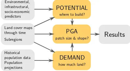
FUTure Urban-Regional Environment Simulation is a stochastic, patched-based model for projecting landscape patterns of urban growth (Meentemeyer et al., 2013). FUTURES has a modular structure consisting of 3 main submodels: DEMAND, POTEN-TIAL and PGA (patch-growing algorithm), see Figure 1. Land conversion is driven by projected population demand computed by the DEMAND submodel, and is spatially defined by a prob-ability surface derived by the POTENTIAL submodel from mul-tiple environmental and socio-economic predictors. The popu-lation demand and the effects of land change drivers can vary in space by subregions, such as jurisdictional units, allowing projec-tions across heterogeneous landscape. FUTURES main strength lies in realistically modeling the spatial structure of urban change by growing patches that are parameterized by size and compact-ness and calibrated using historical data. For a detailed explana-tion of FUTURES’ components, please refer to Meentemeyer et al. (2013).
Figure 1: Simplified schema of FUTURES conceptual model with inputs and outputs in gray and submodels in yellow
The original implementation of FUTURES consisted mainly of the patch-growing algorithm, a standalone program written in a mixture of C and C++. The PGA program itself utilized ineffi-cient algorithms and required raster data in ASCII format as input leading to very slow initialization. The DEMAND submodel was computed in a spreadsheet and POTENTIAL coefficents were de-rived using R statistical software. No official implementation of these submodels existed so each researcher developed a dif-ferent workflow. This made it difficult for peers to verify each other’s work. Several scripts for calibrating patch characteris-tics derived with FRAGSTATS (McGarigal et al., 2012) existed, however these tools were written in an unnecessarily low-level language for a specific case using the author’s directory layout.
When revising the original implementation of FUTURES we iden-tified several issues which needed to be addressed. First, it is im-portant to follow best practices for scientific computing (Wilson et al., 2014) including use of a versioning system, writing doc-umentation and testing. We also wanted to minimize tasks that had been done manually in order to make the process more ef-ficient and avoid errors that are often difficult to detect. When automating tasks we had to compromise between the flexibility and simplicity of the workflow. We also focused on making FU-TURES scalable so that it can run large scale applications at a relatively fine spatial resolution. Finally, we designed FUTURES to be more user-friendly and easy to test so that anyone can con-fidently apply it to their research.
3. INTEGRATION IN GRASS GIS
GRASS GIS has had a long history as a platform for scientific models (Chemin et al., 2015). As an open source GIS used by
researchers worldwide and one of the founding projects of OS-Geo, GRASS GIS provides a stable environment for the devel-opment of scientific models for studying problems from various domains including geomorphology, hydrology, planetary science, landscape ecology, hazard mapping, archaeology, renewable en-ergy and transportation. Thanks to the numerous scientist and developers who have been involved, GRASS GIS today provides a large spectrum of geospatial modules ranging from basic GIS functionality to highly specialized models. Most of the special-ized tools are not part of standard GRASS GIS installations, but are easily accessible from the add-on repository.
There were multiple reasons for our decision to integrate FU-TURES into GRASS GIS as an add-on. Some of these reasons were specific to FUTURES, but others apply to any spatial, sci-entific model. Integrating a model into GIS gives both users and developers a wide array of standard geospatial tools that simplify the implementation of a model, and streamline pre- and post-processing and visualization. GRASS GIS provides model devel-opers a raster library for highly efficient data reading and writ-ing. This means that FUTURES no longer has to read in ASCII files, significantly reducing time needed for initialization. Fur-thermore, raster data from FUTURES simulations are efficiently compressed. Despite ever increasing disk space, it is still quite important to reduce the file size, especially for stochastic spatio-temporal simulations, which typically generate huge datasets. In order to achieve the best speed performance, most GRASS GIS functionality is implemented in C. Because of this, we could eas-ily integrate FUTURES code, written in a mix of C and C++, without major rewriting. For portability reasons we later decided to use the C99 standard. While C and C++ are the preferred lan-guages for computationally expensive algorithms, GRASS GIS also supports Python as the primary scripting language. This is crucial because FUTURES had many steps of data prepara-tion that we were easily able to automate using Python scripting. Model developers can appreciate GRASS GIS’ automatic gener-ation of command line interfaces, Python interfaces and graph-ical user interfaces (GUI). Simply by defining options in C or Python modules we can call the same module from a GUI dia-log, a Python script or a Bash script. A graphical interface makes FUTURES easy to use, especially for users on the Windows plat-form. A Python or Bash interface, however, is needed for more advanced applications such as running FUTURES in parallel on a high performance computer. GRASS GIS provides infrastructure for publishing and distributing models to users on all major plat-forms. Models and tools in GRASS GIS’s Add-on repository1 can be easily browsed and installed with their documentation, re-lieving researchers of the burden of maintaining such infrastruc-ture.
3.1 Implementation
We implemented FUTURES as a set of GRASS GIS modules starting with a common prefixr.futures:
• r.futures.demandextrapolates the area of developed land from population trends and projections.
• r.futures.devpressurecomputes the development pressure pre-dictor.
• r.futures.potentialmodels the development probability sur-face through multi-level logistic regression.
• r.futures.calibcalibrates patch sizes and shapes.
• r.futures.pgasimulates urban development using the patch growing algorithm.
1
In addition, we implemented the add-onr.sample.categoryneeded for the workflow. Since its functionality is not specific to FU-TURES, we kept it separate. All of these add-ons can be conve-niently installed from GRASS GIS using the GUI or command line2. Each individual add-on has a manual page accessible both online and offline. Figure 2 shows FUTURES workflow and the inputs needed for each tool. In the following sections we de-scribe the developed tools, their functionality and implementation in GRASS GIS.
Figure 2: Diagram of FUTURES workflow showing how are r.futuresmodules (yellow boxes) chained and what are their input data (grey boxes). As indicated by the light yellow box,
moduler.futures.calibcallsr.futures.pga.
3.1.1 r.futures.demand Based on historical land development and population growth, the DEMAND submodel (implemented asr.futures.demand) projects the rate of per capita land consump-tion for each year of the simulaconsump-tion and each subregion. This Python module uses GRASS GIS Python Scripting Library and the NumPy, SciPy and matplotlib libraries for scientific comput-ing to approximate the relation between population and land con-sumption with a statistical model described by a linear, logarith-mic or exponential curve. For example, a logarithlogarith-mic relation means that a growing population requires less developed land per person over time. With enough data points, the module can select the best curve for each subregion based on residuals. The primary outputs are plain text files with tab-separated values representing the number of cells to be converted to developed land each year for each subregion. The module plots the resulting curves and projected points for each subregion (Figure 3) so that the results can be visually inspected. The moduler.futures.demandprovides a fast way to estimate the land demand given a large number of subregions with diverse population trends and thus allows us to quickly explore different population scenarios.
3.1.2 r.futures.devpressure Development pressure is one of the most important predictors of where development is likely to happen. For each cell it is computed as a distance decay func-tion of neighboring developed cells (Meentemeyer et al., 2013). Compared to the tool previously used for computing development pressure, the new Python moduler.futures.devpressureprovides a faster and more efficient implementation by taking advantage of the existing GRASS GIS moduler.mfilterwritten in C for moving window analysis with custom designed matrix filters. By precom-puting the matrix of distances we avoid repeated distance compu-tations resulting in faster processing. Because the new implemen-tation is less memory intensive it can be used for larger regions than the previous tool.
3.1.3 r.futures.potential uses multilevel logistic regression to model development suitability based on environmental, infras-tructural, and socio-economic predictors such as distance to roads or topographic slope. We randomly sample these predictors and
2
Figure 3: An example ofr.futures.demandoutput plot showing the logarithmic relation between population and land consumption for the county with ID 37021. Observed data are
showed as blue dots and predicted data as circles.
the observed change from undeveloped to developed cells to es-timate the coefficients of the multilevel logistic regression. The core of this module is a script in the R language (R Develop-ment Core Team, 2008), which uses the package lme4 (Bates et al., 2015) for fitting generalized linear mixed-effects models and the package MuMIn (Barto, 2015) for automatic model selection. The output file is a plain text file with tab-separated regression coefficients. This script is wrapped in Python for more seamless processing and chaining of modules. The coupling between R, Python and GRASS GIS is intentionally very loose to make the workflow possible in the Windows environment where some of the other, more elegant, options such as rpy23are complicated to use. We performed stratified sampling of observed new develop-ment and predictors using GRASS GIS add-onr.sample.category. Although we developed this add-on for urban growth modeling with FUTURES, its application is much broader. In order to en-courage its use in other applications we made it a general module rather than making it part of ther.futurestool set.
3.1.4 r.futures.pga is the main engine of FUTURES – it sim-ulates urban growth using inputs from the DEMAND and PO-TENTIAL submodels. The patch growing algorithm (PGA) sto-chastically allocates a seed for new development across the de-velopment suitability surface, challenges the seed by comparing it with a random number between 0 and 1, and then grows a discrete patch from the seed if it survives (Meentemeyer et al., 2013). This process repeats until the number of converted cells specified by DEMAND is met. The development pressure predic-tor and then the development suitability values are updated based on the newly developed cells. (The development suitability is computed internally from predictors and regression coefficients supplied by POTENTIAL.) We kept the original patch growing algorithm, but significantly improved its implementation to make it faster, more memory efficient and simpler to use. We replaced a custom, undocumented configuration file with a standard module interface usable from GUI or the command line, and restructured the input and output parameters and their names so that they are easy for users to understand. We used efficient GRASS GIS li-braries for reading and writing raster data, which minimized the
3
time needed to initialize the simulation. FUTURES now reads rasters in GRASS’s native format instead of ASCII files. This decreased the time needed for model initialization from several minutes to several seconds for a region with tens of millions of cells. Furthermore, we replaced the static allocation of internal structures with dynamic allocation and reduced the overall mem-ory requirements so that FUTURES could run on large regions with tens or hundreds of counties as well as smaller areas like our case study. Finally, through the use of appropriate programming techniques, such as binary search, we significantly increased the speed of the algorithm.
3.1.5 r.futures.calib We developed a dedicated Python mod-ule for calibrating patch sizes and shapes that runs the modmod-ule r.futures.pgawith different combinations of patch parameters and outputs a table with scores for each combination of patch param-eters. The simulation is run multiple times for each combination to account for the stochasticity of the model. To speed up the calibration processr.futures.calibcan take advantage of multiple computer cores.
4. CASE STUDY
To demonstrate how the new FUTURES framework can be used to simulate urban growth, we present a case study for Asheville metropolitan area located in the Blue Ridge Mountains in the west of North Carolina, USA. The region consists of five counties with total area of 6,271 km2
and around 477,000 people based on 2014 population estimates. It is characterized by rapid popula-tion growth around Asheville, the largest city of the region. New development is constrained by the steep mountainous terrain and large national and state parks. We simulate urban growth from 2012 to 2030 using publicly available data, including the USGS’s National Land Cover Database (NLCD) (Homer et al., 2015, Fry et al., 2011, Homer et al., 2007, Fry et al., 2009), past estimates and future projections of county populations (NCOSBM, 2015), boundaries and roads provided by the United States Census Bu-reau’s database (TIGER) and a digital elevation model from the National Elevation Dataset (NED) distributed by the USGS.
4.1 Approach
There are several steps required to run the FUTURES simulation:
• Preprocess the data.
• Estimate per capita land consumption controlling the total area of converted land.
• Derive the development suitability statistical model to con-trol where the new development happens.
• Calibrate patch size and shape. • Run the urban growth simulation.
4.1.1 Data preparation The core input data for urban growth modeling with FUTURES is a timeseries of land cover maps, which can be derived by various methods from satellite imagery. In this study we used the 2001, 2006 and 2011 NLCD Land Cover products and 1992/2001 Retrofit Land Cover Change prod-uct to derive a 30-meter binary representation of developed areas. We excluded national and state parks, water bodies and wetlands from further analysis. We used NLCD products that are avail-able for the contiguous USA so that this study and its workflow would be easier to reproduce and apply to other study areas. We obtained population statistics from the North Carolina Office of State Budget and Management, which are based on 2000 and 2010 censuses and include past as well as future estimates of pop-ulation per county for each year up to 2035. Data for the 5 coun-ties studied were extracted and formatted as a comma-separated values (CSV) file.
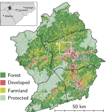
Figure 4: 2011 land cover (Homer et al., 2015) and protected areas (Anderson and Sheldon, 2011) in the Asheville metropolitan area in the west of North Carolina, USA. Inset A is
used in Figure 5.
4.1.2 DEMAND We derived the relation between population
and land consumption from the series of binary rasters of de-veloped areas and population statistics to model how much land will be developed each year of the simulation. Using the mod-uler.futures.demandwe explored different curve fitting methods and derived the per capita land consumption from period 1992 through 2011, which was characterized by population growth with decreasing demand for land per person over time. We expect sim-ilarly low rates of per capita land consumption in the following years because development is restricted by the mountainous ter-rain and large protected areas. Based on RMSE and visual inspec-tion of the plots created byr.futures.demandwe selected either linear or logarithmic relations for each county, where the function coefficients were automatically determined using linear regres-sion and non-linear least squares optimization inr.futures.demand (Figure 3).
subse-undeveloped projected development developed until 2011 protected areas and water
roads 5 km
a) sprawl b) status quo c) infill
Asheville Asheville Asheville
Asheville AshevilleAsheville
Figure 5: Results of three realizations of multiple stochastic runs with different scenarios. Depending on the scenario, simulated development is more diffuse (a) or more compact (c).
quent updates are performed in memory during the simulation.
Predictors Estimate* Std. Error
Intercept (varies by county) -2.593 0.269
Development pressure 0.058 0.005
Road density 0.118 0.007
Percentage of forest -0.013 0.002
Distance to protected areas -0.140 0.039 Distance to water bodies -0.148 0.022
* all P-values<0.001
Table 1: List of selected predictors and estimated coefficients for site suitability model
4.1.4 Patch calibration Prior to running the urban growth simulation implemented inr.futures.pgawe calibrated the input patch compactness and size to match the simulated patterns with the observed patterns from 1992 to 2011. Since calibration is a time consuming process, we ran the moduler.futures.calibfor Buncombe county and applied the results to the rest of our study region. We choose Buncombe County which includes the city of Asheville because it is where most new development will oc-cur. For each combination of patch parameters we compared the patch characteristics averaged from 20 runs of the urban growth simulation with the known patches. Based on the score we se-lected patch parameters resulting in high compactness which is expected for mountainous regions.
4.1.5 Urban growth simulation Having collected all neces-sary input data, we ranr.futures.pgawith a 1 year time step until 2035 for the entire study region at 30 m resolution. To account for different future policies regarding new development, we explored scenarios altering the site suitability to encourage infill or sprawl by changingincentive powerparameter ofr.futures.pga. This value transforms the probabilitypa cell is developed topxwhere x= 1represents status quo, higher values ofxresult in infill and
lower values in sprawl. In addition to the status quo we simulated scenarios withxequals 0.25, 0.5, 2 and 4. We repeated each
scenario 50 times to account for the model’s stochastic behavior.
4.2 Results
The resulting development patterns of three realizations of the random runs are visible in Figure 5 for the status quo, infill sce-nario (x= 4) and sprawl scenario (x= 0.25). The simulated
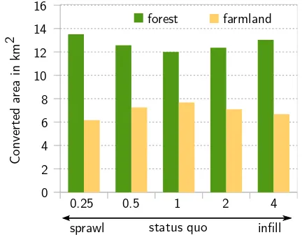
patches realistically mimic the current patches of development in shape and size and are mostly, but not exclusively adjacent to roads as expected. Furthermore, we post-processed the results to study how different urban growth policies influence the loss of forest and agricultural land in the Asheville area (Figure 6) by averaging the loss of both land use categories over the 50 runs. In all scenarios, forest is more affected by future development than farmland. The extreme case of urban sprawl results in twice as much forest as farmland being developed. Status quo scenario leads to the smallest difference between the areas converted to forest and farmland. Interestingly, infill scenario develops the forested area in a similar way as sprawl does, which is not surpris-ing considersurpris-ing developed areas are largely surrounded by forest patches.
0.25 0.5 1 2 4
0 2 4 6 8 10 12 14 16
forest farmland
infill
sprawl status quo
C
on
ve
rt
ed
a
re
a
in
k
m
2
Figure 6: Area in km2of converted land from forest (green) and farmland (yellow) to urban differs for urban sprawl and infill scenarios. Numbers0.25to4represent the exponentxwhich
transforms development probabilityptopx.
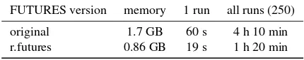
Shavit, 2012) in which the computation can easily be distributed across multiple computer cores.
FUTURES version memory 1 run all runs (250)
original 1.7 GB 60 s 4 h 10 min
r.futures 0.86 GB 19 s 1 h 20 min
Table 2: Time and memory needed to run the simulations with the old version of FUTURES and the newr.futuresimplemented
in GRASS GIS on a laptop with 64-bit Ubuntu 14.04 LTS, Intel Core [email protected] using 1 CPU and running on
external hard drive.
The input data and instructions to run the model are available as part of material developed for the US-IALE 2016 Annual Meet-ing workshop on FUTURES4.
5. DISCUSSION
The new FUTURES framework is split into independent GRASS GIS modules so that the modeling workflow is flexible and ex-tendable. By using standardized inputs and outputs (raster lay-ers and CSV files) and described interface we allow FUTURES’ users to replace DEMAND and POTENTIAL implementations by their own tools, which may be better suited to the character-istics and datasets available for their study systems. We ran all previous studies on county level at 30 m resolution. FUTURES, however, can be applied to larger or smaller scales as long as there is data available and the patch characteristics are properly calibrated. Future research will explore nested scales in order to address the different scales of the population data and the spatial drivers of land change.
6. CONCLUSION
We presented a new, open source version of the FUTURES ur-ban growth model that is integrated into GRASS GIS, opening new possibilities for environmental scientists and urban planners to project and understand the impacts of urbanization at relevant ecological and decision-making scales. Integration into GRASS GIS allowed us to make FUTURES more efficient, simple to use and transparent. With documented code running on all platforms, FUTURES can now be easily tested and applied to study sites at local to megaregional scales. We illustrated how FUTURES can be used in a small case study of the Asheville metropolitan area. We also provided the instructions and data needed to reproduce this study as a step towards more reproducible research in land change science.
ACKNOWLEDGEMENTS
We would like to thank Monica Dorning and Douglas Shoemaker for discussing with us the original model implementation, and Brian Pickard and Georgina Sanchez for testing new FUTURES implementation.
REFERENCES
Alberti, M., 2005. The effects of urban patterns on ecosystem function. International regional science review28(2), pp. 168– 192.
4
https://grasswiki.osgeo.org/wiki/Workshop_on_urban_ growth_modeling_with_FUTURES
Anderson, M. and Sheldon, A. O., 2011. Conservation Status of Fish, Wildlife, and Natural Habitats in the Northeast Land-scape: Implementation of the Northeast Monitoring Framework. Technical report, The Nature Conservancy, Eastern Conservation Science.
Barto, K., 2015. MuMIn: Multi-Model Inference. R package version 1.15.1.
Bates, D., Maechler, M., Bolker, B. and Walker, S., 2015. lme4: Linear mixed-effects models using Eigen and S4. R package ver-sion 1.1-9.
Chaudhuri, G. and Clarke, K. C., 2013. The sleuth land use change model: A review.International Journal of Environmental Resources Research1(1), pp. 88–104.
Chemin, Y., Petras, V., Petrasova, A., Landa, M., Gebbert, S., Zambelli, P., Neteler, M., L¨owe, P. and Di Leo, M., 2015. GRASS GIS: a peer-reviewed scientific platform and future re-search repository. In: Geophysical Research Abstracts, Vol. 17, p. 8314.
Dorning, M. A., Koch, J., Shoemaker, D. A. and Meentemeyer, R. K., 2015. Simulating urbanization scenarios reveals tradeoffs between conservation planning strategies.Landscape and Urban Planning136, pp. 28–39.
Easterbrook, S. M., 2014. Open code for open science? Nature Geoscience7(11), pp. 779–781.
Fry, J., Coan, M., Homer, C., Meyer, D. and Wickham, J., 2009. Completion of the National Land Cover Database (NLCD) 1992– 2001 Land Cover Change Retrofit Product. Technical report, U.S. Geological Survey Open-File Report 20081379.
Fry, J., Xian, G., Jin, S., Dewitz, J., Homer, C., Yang, L., Barnes, C., Herold, N. and Wickham, J., 2011. Completion of the 2006 National Land Cover Database for the Conterminous United States. PE&RS77(9), pp. 858–864.
Herlihy, M. and Shavit, N., 2012.The Art of Multiprocessor Pro-gramming, Revised Reprint. Elsevier.
Homer, C., Dewitz, J., Fry, J., Coan, M., Hossain, N., Larson, C., Herold, N., McKerrow, A., VanDriel, J. and Wickham, J., 2007. Completion of the 2001 National Land Cover Database for the Conterminous United States. Photogrammetric Engineering and Remote Sensing73(4), pp. 337–341.
Homer, C., Dewitz, J., Yang, L., Jin, S., Danielson, P., Xian, G., Coulston, J., Herold, N., Wickham, J., and Megown, K., 2015. Completion of the 2011 National Land Cover Database for the conterminous United States – Representing a decade of land cover change information. Photogrammetric Engineering and Remote Sensing81(5), pp. 345–354.
Jantz, C. A. and Goetz, S. J., 2005. Analysis of scale dependen-cies in an urban land-use-change model.International Journal of Geographical Information Science19(2), pp. 217–241.
McGarigal, K., Cushman, S. and Ene, E., 2012. FRAGSTATS v4: spatial pattern analysis program for categorical and continuous maps. Computer software program produced by the authors at the University of Massachusetts, Amherst.
Meentemeyer, R. K., Tang, W., Dorning, M. A., Vogler, J. B., Cunniffe, N. J. and Shoemaker, D. A., 2013. FUTURES: Multi-level Simulations of Emerging UrbanRural Landscape Structure Using a Stochastic Patch-Growing Algorithm. Annals of the As-sociation of American Geographers103(4), pp. 785–807.
Neteler, M. and Mitasova, H., 2008.Open Source GIS: A GRASS GIS Approach. Vol. 773, Springer, New York.
Pickard, B. R., Van Berkel, D., Petrasova, A. and Meentemeyer, R. K., in prep. Future patterns of urbanization reveal trade-offs among ecosystem services.
R Development Core Team, 2008. R: A Language and Envi-ronment for Statistical Computing. R Foundation for Statistical Computing, Vienna, Austria. ISBN 3-900051-07-0.
Shoemaker, D. A., 2016. The role of spatial heterogeneity and urban pattern in modulating ecosystem services. Doctoral dissertation, North Carolina State University. Retrieved from http://www.lib.ncsu.edu/resolver/1840.16/11033.
Sohl, T. L., Sayler, K. L., Drummond, M. A. and Loveland, T. R., 2007. The FORE-SCE model: a practical approach for projecting land cover change using scenario-based modeling. Journal of Land Use Science2(2), pp. 103–126.
Verburg, P. H., Soepboer, W., Veldkamp, A., Limpiada, R., Espal-don, V. and Mastura, S. S., 2002. Modeling the spatial dynamics of regional land use: the CLUE-S model. Environmental man-agement30(3), pp. 391–405.
Waddell, P., 2002. UrbanSim: Modeling urban development for land use, transportation, and environmental planning.Journal of the American Planning Association68(3), pp. 297–314.