COMPARISON OF POINT MATCHING TECHNIQUES FOR ROAD NETWORK
MATCHING
A. Hackeloeer a,K. Klasing a, J. M. Krisp b, L. Meng b
a BMW Forschung und Technik GmbH, Hanauer Straße 46, 80992 Munich, Germany – (andreas.hackeloeer, klaas.klasing)@bmw.de
b Department of Cartography, Technische Universität München, Arcisstraße 21, 80333 Munich, Germany – (jukka.krisp, liqiu.meng)@bv.tu-muenchen.de
KEY WORDS: Conflation, Road Network Matching, Point Matching
ABSTRACT:
Map conflation investigates the unique identification of geographical entities across different maps depicting the same geographic region. It involves a matching process which aims to find commonalities between geographic features. A specific subdomain of conflation called Road Network Matching establishes correspondences between road networks of different maps on multiple layers of abstraction, ranging from elementary point locations to high-level structures such as road segments or even subgraphs derived from the induced graph of a road network.
The process of identifying points located on different maps by means of geometrical, topological and semantical information is called point matching. This paper provides an overview of various techniques for point matching, which is a fundamental requirement for subsequent matching steps focusing on complex high-level entities in geospatial networks. Common point matching approaches as well as certain combinations of these are described, classified and evaluated. Furthermore, a novel similarity metric called the Exact Angular Index is introduced, which considers both topological and geometrical aspects. The results offer a basis for further research on a bottom-up matching process for complex map features, which must rely upon findings derived from suitable point matching algorithms. In the context of Road Network Matching, reliable point matches provide an immediate starting point for finding matches between line segments describing the geometry and topology of road networks, which may in turn be used for performing a structural high-level matching on the network level.
1. INTRODUCTION
Conflation can be seen as the process of identifying geographical entities across different maps depicting the same geographic region which are then combined to create a new map. According to a definition proposed by Longley et al. [1],
conflation is „the process of combining geographic information from overlapping sources so as to retain accurate data, minimize redundancy, and reconcile data conflicts”. A classification approach introduced by Yuan and Tao [2] divides conflation into horizontal (combining neighboring areas) and vertical conflation (combining different maps of the same area). Throughout this paper, we will focus on vertical conflation, while most point matching techniques are applicable to both types.
In general, three different types of information can be used in the conflation process: geometrical, topological, and semantical. Geometrical information describes geometric properties of an object, such as the shape of a road segment. Topological information is exposed by the graph structure induced by networks of certain geographical objects, such as roads or rivers. Semantical information can be seen as any kind of information which does not belong to the other two categories; e.g., street names belong to this category.
Both raster image as well as vector data may be used for conflation. However, different conflation strategies are required depending on the type and direction (to-raster [3], raster-to-vector [4], vector-to-raster [5], or vector-raster-to-vector [6]). Throughout this paper, we will focus on vector-to-vector pairings of maps.
A specific subdomain of conflation called Road Network Matching [7] investigates correspondences between road networks of different maps, which may be established on different levels, ranging from elementary point locations to complex aggregated structures such as sequences of road segments. All mentioned types of information can be considered for each of these levels. A common approach in the domain of Road Network Matching involves a bottom-up matching strategy [8] which starts with point matching, i.e. finding relations between point locations. These matching results are then further processed in order to provide a basis for higher-level matchings between aggregated structures such as road segments.
This work is concerned with introducing, classifying and evaluating point matching techniques for Road Network Matching. The overview (Section 2) describes the point matching problem in general. Section 3 gives a classification of point matching techniques based on the type of information considered and describes the different approaches in detail, including a novel approach named Exact Angular Index. In Section 4, the described point matching techniques are evaluated with respect to properties such as accuracy and complexity in a real-world scenario involving maps from different sources such as OpenStreetMap. Section 5 summarizes the results. We therefore intend to provide the reader with a quick understanding of the advantages and disadvantages of the presented point matching techniques, which offer a starting point for identifying higher-level matchings required within the Road Network Matching process.
2. OVERVIEW OF THE POINT MATCHING PROBLEM
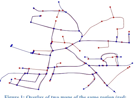
Figure 1 shows a road map of the village of Moosach, near Munich, Germany, provided by the Bavarian State Office for Survey and Geoinformation, Munich [9], which is called ATKIS Basis-DLM. This area is overlaid with a road map built from geographic data provided by the Volunteered Geographic Information (VGI) project OpenStreetMap (OSM).
Figure 1: Overlay of two maps of the same region (red: ATKIS, blue: OSM)
Topologically, each map consists of a graph (the road network) given by edges and nodes (vertices), where a node represents a geographical point referenced via its coordinates in a suitable reference system (e.g. WGS-84), and an edge is given by a relation which describes a connection between two nodes. For the purposes of point matching, the graph may be seen as being undirected to simplify the process. It should be noted that many map providers insert bivalent nodes (nodes which are only incident to two edges) at locations where attributes change which are recorded per edge. Occasionally, the terms 0-cells for nodes, 1-cells for edges, and, subsequently, 2-cells for polygons consisting of a sequence of edges are used [10].
Geometrically, the shape of a road segment represented by an edge in the graph is described via shape points (not explicitly shown in the figures), where a sequence of shape points constitutes the geometrical layout of the road segment corresponding to an edge. Like nodes, shape points are defined by their coordinates. Continuous shape geometry is created by employing linear interpolation between shape points.
While it is possible to employ point matching strategies to any data consisting of spatial point coordinates, such as Points of Interest (POIs) or shape points, matching topological nodes in a road network is of special concern for the domain of Road Network Matching. The following boxes give a formal definition of solutions to the point matching problem for two road networks with respect to topological nodes.
Notes:
- A solution according to Def. 2 represents an M:N type mapping between nodes of � and �.
- A left-unique solution according to Def. 3 represents a 1:N type mapping between nodes of � and �. - A right-unique solution according to Def. 4 represents
a N:1 type mapping between nodes of � and �. - A unique solution according to Def. 5 represents a 1:1
type mapping between nodes of � and �. - A complete solution only exists if |� | = |� |.
As can be seen in Figure 1, several problems surface when dealing with the point matching problem in real-world scenarios:
1. Topological differences:
The two maps do not share the same topology. Rather, roads are present in one map which are missing in the other map. Also, due to a varying level of detail, even roads present in both maps may be modelled with a different number of nodes. In addition, structures such as complex intersections may be modelled differently, resulting in a different placement of nodes.
2. Geometrical differences:
Due to varying accuracy in the recorded coordinates, the geographical location of nodes representing the same topological entity may differ between the maps to a great extent. On the other hand, nodes in close proximity do not necessarily imply a topological relationship.
3. Semantical differences:
Nodes may carry semantical information, such as the names of incident roads. While semantical similarity of two nodes in different maps often indicate that the same node is referenced, semantical dissimilarity rarely implies the opposite, since semantical attributes as well as the extent to which they are recorded vary greatly across different map providers and sources. E.g., street names may be spelled differently, and there may also be multiple names for the same street.
In order to deal with these problems, several algorithms have evolved which determine and evaluate point matching
DEFINITION 2:SOLUTION TO THE POINT MATCHING PROBLEM FOR TWO ROAD NETWORKS.
A solution to the point matching problem for two road networks is a relation ⊆ � × � , i.e., a set of point matchings.
DEFINITION 3: LEFT-UNIQUE SOLUTION TO THE POINT
MATCHING PROBLEM FOR TWO ROAD NETWORKS.
A left-unique solution to the point matching problem for two road networks is an injective relation ⊆ � × � .
DEFINITION 4: RIGHT-UNIQUE SOLUTION TO THE POINT
MATCHING PROBLEM FOR TWO ROAD NETWORKS.
A right-unique solution to the point matching problem for two road networks is a functional relation ⊆ � × � .
DEFINITION 5:UNIQUE AND COMPLETE SOLUTIONS TO THE
POINT MATCHING PROBLEM FOR TWO ROAD NETWORKS.
A unique solution to the point matching problem for two road networks is a right-unique and left-unique relation �⊆ � × � . Note that is a unique solution. If � is also surjective and left-total, it is a complete solution.
DEFINITION 1:POINT MATCHING FOR TWO ROAD NETWORKS. Given are two undirected simple graphs � , � representing a road network: � = � , � , � { , }, where � is the set of vertices of graph �, and � the edge relation of Graph �, and � ⊆ � × � . Then, a point matching is a pair
, , where � and �.
candidates (i.e., a subset of all point matchings) with respect to certain metrics. In general, a metric is defined as follows:
Thus, in the context of the point matching problem, a metric is a distance function which assigns a real number to a point matching, where the assigned value expresses the degree of dissimilarity of the two points involved. The distance may be normalized, e.g. by projecting it onto the interval ; ], where 1 corresponds to the lowest possible distance (0, meaning equality) and 0 corresponds to an infinitely high distance. We call such a projection a score, because it is positively correlated with the expected quality of the matching from the perspective of the according metric. The overall score which an algorithm attributes to a point matching may be a weighted combination of multiple scores from different metrics.
In order to limit the computational effort, point matching algorithms usually only evaluate a small subset of all possible point matchings. Most point matchings are discarded beforehand due to spatial constraints, since it is assumed that the probability of two points representing the same spatial entity quickly becomes extremely low as the distance between the points increases beyond several kilometres. The fact that point matching algorithms, unlike pure graph matching approaches, may not only rely on topological but also on geometrical information thus greatly simplifies the point matching problem, since it reduces the number of candidates which need to be evaluated.
While a complete solution as defined in Def. 5 may seem desirable, it only exists for very simple scenarios where the two maps being compared are virtually identical (e.g., very minor map updates). In real-world applications, usually both maps contain several nodes which cannot reasonably be matched to the other map.
Point matching algorithms deliver a set of point matchings, where each point matching is assumed to identify the same geographical entity across both maps. This is done by evaluating the degree of similarity between point matchings close enough to become candidates according to certain metrics, then selecting those point matchings for the solution which are considered similar enough that they may reasonably represent the same spatial feature (e.g. by applying a global or local threshold on the score). In general, this solution is ambiguous, implying that any point on any of the two maps may be matched to more than one point in the other map. It is possible to establish unique solutions by discarding all matchings related to a node except the highest-rated point matching. However, in special cases, a geographical entity represented by one topological node in one map may be (partially) represented by multiple nodes in the other map (e.g. bivalent nodes, differing level of detail, or complex intersections), so these cases must be recognized and dealt with separately.
3. CLASSIFICATION AND DESCRIPTION OF POINT MATCHING TECHNIQUES
Point matching techniques may be based on geometrical, topological, or semantical information, or a combination of these three. Since most map providers do not include semantic
attributes for topological nodes and semantical matching techniques referring to incident edges are more appropriate for edge matching, we will not discuss semantical matching in greater detail.
3.1 Geometrical point matching techniques
Geometrical point matching techniques only consider geometrical information (i.e., coordinates) for evaluating a point matching. Even though the distance between point coordinates may be calculated in any p-norm, the only metric of practical relevance is the Euclidean distance metric.
3.1.1 Pure Euclidean
Obviously, spatial proximity is a strong constraint for the selection of matching candidates. In the Euclidean plane, the distance dist , of two points = , and = , is given by
dist , = √ − + − ².
While for small geographical regions, Euclidean geometry is a good approximation, a more exact measure for the distance between two points on the surface of the Earth is the great-circle distance, which describes the shortest distance between any two points on the surface of a sphere following a path on the surface. The great-circle distance can be computed using the spherical law of cosines or the numerically better-conditioned Haversine formula [11]. The approaches presented in this paper use a Euclidean distance metric applied to a Universal Transversal Mercator (UTM) projection of WGS-84 coordinates for calculating distances, as it provides sufficient accuracy and can be computed efficiently.
A naïve approach to conduct Pure Euclidean point matching calculates the Euclidean distance dist , for each point matching pair ( , ) � × � which possesses all properties of a metric function as defined in Def. 6. To extract a right-unique solution , each � is assigned to a � where � , becomes minimal so that , and
, ≠ ∀ �. In order to gain a left-unique solution , each � may only be related to a � where � , becomes minimal so that , and
≠, ∀ � . Finally, a unique solution �= can be derived.
This approach is obviously inefficient as it evaluates every possible point matching pair. However, by employing a spatial index (e.g. a kd-tree) and only evaluating neighbors within a sufficiently large radius, Pure Euclidean matching may be performed efficiently without losing substantial accuracy.
The Euclidean distance may be projected to a score of the interval (0; 1] by using the following formula:
scorePE( , ) =
+ dist( , ) ²
where ℝ+ is a correction factor and ℝ+ is the node search radius. Note that lim
dist→∞score( , ) = for any , . 3.2 Topological point matching techniques
Topological point matching techniques employ topological information such as the valence (number of incident edges) per node.
DEFINITION 6:METRIC DEFINITION FOR POINT MATCHING. A metric on a set � ≔ � � is a function : � × � → ℝ where ∀ , , �, these conditions must be satisfied:
(a) , = ⟺ =
(b) , = ,
(c) , ≤ , + ,
3.2.1 Node Valence
The valence, or degree, of a node in a graph is defined as the number of edges incident to the node, where loops are counted twice.
The Node Valence point matching approach is concerned with the differences in valence found between the two nodes of a point matching. The larger this difference grows, the lower the probability becomes that both nodes reference the same geographical entity. However, minor differences in valence are no guarantee that the nodes are a bad matching, since the two maps may differ in actuality or level of detail so that e.g. small roads may only be present in one map. Also, equal valence does not imply node equality, so that node valence on its own does not qualify as a metric, since it violates condition (a) in Def. 6.
The valence difference may be combined with the Euclidean distance to obtain an order in case of equal valence difference. Since point matchings of large geometrical distances are unlikely to represent a proper solution, the search for matching candidates regarding a node may be limited to its neighborhood within a certain radius. Only within this neighborhood, node valence needs to be evaluated. The lower the difference of valence is, the higher the assumed similarity of two nodes. If two matching candidate pairs are assigned to the same equivalence class regarding their valence difference, the pair with the lower Euclidean distance is assumed to be more similar. Depending on properties of the maps to be matched such as node density or dispersion, Node Valence may require a fine-tuning of the search radius to provide acceptable solutions.
A straightforward approach for calculating a score based on valence difference is reflected by the following formula:
scoreNV( , ) =
+ |val − ( )|
3.3 Combined geometrical / topological point matching techniques
Combined geometrical / topological point matching techniques are employed by algorithms which follow both geometrical as well as topological approaches and combine them in order to achieve better matching results.
3.3.1 Spider Index
Rosen and Saalfeld [10] describe a point matching technique called the Spider Index, which overlays a node with a circular 8-sector discretization of 45° angle intervals similar to a compass rose. Each sector corresponds to one bit within an 8-bit number. A bit is set to true if and only if there is an incident edge that falls into the corresponding sector. Thus, each node can be described by an 8-bit number with bits �1⋯ �8. For two nodes � and � the score of the spider index is then calculated as
scoreSI= 8∑�( �, �), 8
=
where �( �, �) = � ↔ � is the binary equivalence function, i.e. � = if bits are equal and � = if they are different. Note that we have normalized the score to the interval [0; 1].
Due to the information loss resulting from the quantization, two nodes may still be considered equal if the angles of their incident edges are different within the limits of a sector. Moreover, it may happen that two nodes are not considered equal if the angles of their incident edges are rotated by a tiny
degree, but beyond the limits of a sector. Yet, compared to Node Valence, the Spider Index offers a more accurate measure for node equality, as it not only accounts for topological valence difference, but also geometrical angle difference.
As with Node Valence, the Spider Index alone does not qualify as a metric, since two matching candidate pairs whose bit difference regarding their Spider Index is zero may still be different. However, in the same way as with Node Valence, the Spider Index may be turned into a metric by combining it with the Euclidean distance, so that Euclidean distance determines an order where the Spider Index does not discriminate.
3.3.2 Exact Angular Index
Here, we introduce a novel similarity metric called the Exact Angular Index (EAI). Like the Spider Index, the EAI aims to find point matching solutions which consider both topological valence and geometrical angle difference of incident edges. However, the EAI does not employ quantization. Rather, the best mapping between the edges of the two nodes of a matching candidate, i.e. the mapping which minimizes the angle differences between the vectors derived from the geometrical shapes of the edges, is determined by evaluating all possible edge mappings. Then, a score is calculated based on the sum of minimum angle differences according to the mapping relative to the largest possible sum of angle differences, where differences in valence are counted as the worst possible angle differences.
Formally, the algorithm follows these steps to iteratively assign a score to point matchings {( , )| � , � } for each
with incident edges � ⊆ �:
- For each incident edge of , calculate the geographical heading, i.e. the angle between the vector given by the first linear segment of the edge and true north in clockwise direction. The result is a heading function ℎ : � → ℝ.
- Search for nodes , . . , � � in � within a fixed radius around the position of . If no surrounding nodes can be found, no matching partner can be assigned to , so the algorithm continues with the next node + .
- For each found node � with incident edges � ⊆ � : 1. Calculate the heading function ℎ : � → ℝ.
2. Calculate the best-mapping function : � → � which determines the optimum mapping from each edge incident to to an edge incident to regarding their angle difference, using ℎ and ℎ . If |� | > |� |, there are edges �
�
̅̅̅̅ ⊆ � which could not be mapped to edges of � and = ∅ ∀ �
� ̅̅̅̅. 3. Calculate the sum of all angle differences all by
adding up the differences between the headings of all best-mappings gained from :
all= ∑ Δ ℎ , ℎ ( )
�
=
where ≤ ≤ �, { , . . , �} ⊆ � �̅̅̅̅� and Δ , is the angle difference computed by Δ , =
mod | − |, 6 .
4. If there is a difference in valence between and , add an angle difference of 180° per missing or redundant edge to get the normalized sum of all angle differences norm:
norm= all+ 8 |val − val( )|
where val is the valence of node . 5. Calculate the largest possible sum of angle differences
largest:
largest= 8 max val ,val( ) Then project the quotient of norm and largest onto a score in the interval of [0; 1] which expresses the degree of similarity by subtracting it from 1:
scoreEAI( , ) = − norm
largest The best-mapping function employs a queue for edges = { , . . , �} ⊆ � which are not mapped yet, a mapping relation � ⊆ � × � holding established mappings, a
record function : � → � , ℝ storing the best angle
difference found for a destination edge found so far along with its source edge, and an angle difference function
ad : � , � → ℝ, , ↦ Δ (ℎ , ℎ ).
Initially, = � , � = ∅ and = ∅, ∞ ∀ � . The
algorithm then repeats the following steps until = ∅: 1. Take one edge from queue so that ≔
{ }.
2. Get sorted list , . . , � of angle differences between and each incident to using ad . Also store the assignment between and as
function ea: ℕ → � , � ↦ .
3. For each ,ea � : Iteratively verify record
ea � = old, ∂old . If < ∂old, enqueue old ≔ { old} , update ea � ≔ ( , ), and leave iteration (since everything that follows would be a worse assignment, as the list is sorted). Otherwise, proceed until a new difference record has been found or there are no differences left.
If = ∅, add all projections of = , to � � ≔
� { , }) where ≠ ∅, ∞ . Then, M holds the
optimum mapping and the algorithm terminates.
3.3.3 Exact Angular Index + Distance
It is possible to calculate a weighted score scorew , which incorporates both the Exact Angular Index as well as the Euclidean distance with the following formula:
scorew( , ) = scoreEAI( , ) +
scorePE ,
where = | − | [ ; ] ⊆ ℝ describes the weight given to the topological similarity of the nodes expressed by the EAI score, and = | − | [ ; ]⊆ ℝ stands for the weight given to the geometrical similarity of the nodes expressed by the Pure Euclidean score.
4. EVALUATION OF POINT MATCHING TECHNIQUES
In the previous section, several point matching techniques were introduced. In order to evaluate these approaches, we employ an experimental setup involving real-world road maps. At first, we create a unique matching solution serving as a ground truth by manually assigning matches. Matching results of the different point matching techniques are then compared to the ground truth assignments. This way, accuracy and performance can be measured and discussed.
4.1 Experimental Setup
We investigated the point matching approaches described in section 3 using samples from two regions: The village of Moosach, Germany, as seen in Figure 1 serves as an example
for relatively simple matching problems (Area: 590000 m², 54 nodes in reference map, 100 nodes in matching map, boundaries [48.036587,11.870445 | 48.029227,11.880119]), and a part of the inner city of Munich, Germany is used as an example for difficult matching cases (Area: 81800 m², 26 nodes in reference map, 39 nodes in matching map, boundaries [48.151872, 11.5543 | 48.149853, 11.559203]). For the Moosach region, our sources were OpenStreetMap and a commercial map vendor, and a search radius of 40 meters was set. For the sample of the inner city of Munich, we employed the ATKIS Basis-DLM map as well as OpenStreetMap data, using a search radius of 20 meters due to the higher density of nodes. For each region, we manually created a ground truth matching reflecting the best association of nodes by visual inspection (Moosach: 37 matching pairs, Munich: 17 matching pairs). Each point matching algorithm was applied to each pairing of maps, then we compared the results to the ground truth matching in order to evaluate the number of true positives (matching pairs found in the ground truth), false positives (matching pairs not found in the ground truth), and false negatives (matching pairs present in the ground truth, but missing in the matching result generated by the algorithm). We also investigated the correlation between the score of a point matching pair and the probability of it being a true positive, in order to derive a threshold for acceptable matchings. All discussed results refer to unique solutions according to Def. 5.
4.2 Results
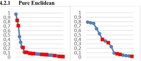
4.2.1 Pure Euclidean
Figure 2: Pure Euclidean Scores for a simple (left, Moosach) and a complex (right, Munich City) region
Figure 2 shows decreasing matching scores of Pure Euclidean Matching. False positives are marked as red squares. Of the 37 matching pairs defined by the ground truth matching for the Moosach sample, 26 (70%) were correctly identified. There were 15 false positives and 11 false negatives. The complex sample yielded slightly worse results: 11 (65%) correct matching pairs, 5 false positives, and 6 false negatives. Since false positives seem to be evenly distributed among the scores, a safe threshold for discarding bad matchings must be set at the very end of the scale.
4.2.2 Node Valence
Figure 3: Node Valence Scores for a simple (top) and a complex (bottom) region
The scores of Node Valence Matching can be seen in Figure 3. Node Valence was able to correctly identify 34 matching pairs
0 0,1 0,2 0,3 0,4 0,5 0,6 0,7 0,8 0,91
0 0,1 0,2 0,3 0,4 0,5 0,6 0,7 0,8 0,91
0,3 0,5 0,7 0,9
0,3 0,5 0,7 0,9
(92%) [7 FP, 3 FN] in the simple region and 14 matching pairs (82%) [1 FP, 3 FN] in the complex region. Clearly, node valence alone is a very coarse measure, thus a reasonable threshold for acceptable matchings cannot be established. 4.2.3 Spider Index
Figure 4: Spider Index Scores for a simple (top) and a complex (bottom) region
The Spider Index (scores shown in Figure 4) identified 33 matching pairs found in the ground truth (89%) in the simple region [8 FP, 4 FN] and 10 matching pairs (59%) [6 FP, 7 FN] in the complex region. The resolution of the score is so low that for (nearly) all of the 8 possible score values, true as well as false positives were found, and thus, no threshold could be derived.
4.2.4 Exact Angular Index
Figure 5: Exact Angular Index Scores for a simple (top) and a complex (bottom) region
Within the simple region, the Exact Angular Index (Figure 5) identified 33 true positives (89%) [8 FP, 4 FN], and within the complex region, 12 true positives (71%) [3 FP, 5 FN]. Contrary to the Spider Index, the scores found provide a basis for establishing a threshold, as high scores are clearly, though not perfectly, correlated with true positives. In the both of the samples shown, an acceptance threshold of 0.8 offers a balanced compromise which selects the most true positive matchings while rejecting most false positives.
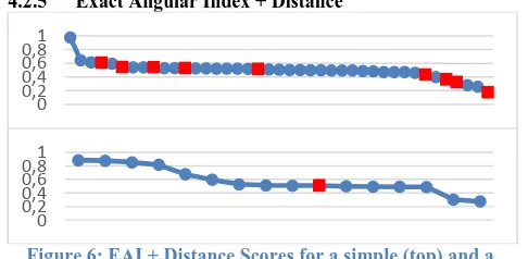
4.2.5 Exact Angular Index + Distance
Figure 6: EAI + Distance Scores for a simple (top) and a complex (bottom) region
The combination of the EAI score with Euclidean distance with a weight of 50% for each component yielded 32 true positives (82%) [9 FP, 5 FN] in the simple region and 15 true positives (88%) [1 FP, 2 FN] in the complex region (Figure 6). For the first sample, Euclidean distance deteriorates the matching accuracy of the Exact Angular Index, to an extent where a safe threshold can no longer be derived. Thus, for this sample, it can be stated that topological similarity should be preferred over
geometrical distance in order to achieve good matching results. However, for the complex region, the matching result is the best of all algorithms discussed here regarding sensitivity as well as specificity.
5. SUMMARY
In this paper, we have provided an overview of different point matching techniques for road network matching. We classified and described several point matching algorithms in detail, including a novel matching algorithm called Exact Angular Index, which offers an exact metric for the topological similarity of nodes in a road network. Finally, we presented an experimental evaluation of the point matching algorithms using real-world maps of two different regions from multiple sources. The results show that especially for complex matching cases, combinations of topological and geometrical approaches provide an advantage in both accuracy and precision, while maintaining acceptable execution times.
6. REFERENCES
[1] P. A. Longley, M. F. Goodchild, D. J. Maguire and D. W. Rhind, Geographic Information Systems and Science, John Wiley & Sons, 2005.
[2] S. Yuan and C. Tao, "Development of Conflation Components," in International Symposium of Geoinformatics and Socioinformatics and Geoinformatics, Ann Arbor, Michigan, 1999.
[3] W. Christmas, J. Kittler and M. Petrou, "Matching of road segments using probabilistic relaxation: a hierarchical approach," in Neural and Stochastic Methods in Image and Signal Processing III, vol. SPIE 2220, San Diego, CA, USA, Chen, S.-S., 1994, pp. 166-174.
[4] D. G. O'Donohue, “Matching of image features and vector objects to automatically correct spatial
misalignment between image and vector data sets,” 2010.
[5] B. Kovalerchuk, P. Doucette, G. Seedahmed, R. Brigantic, M. Kovalerchuk and B. Graff, "Automated vector-to-raster image registration," Proceedings of SPIE, vol. 6966, pp. 69660W-1-69660W-12, 2008.
[6] G. Gösseln, "A matching approach for the integration, change detection and adaptation of heterogeneous vector data sets," in XXII International Cartography Conference, 2005.
[7] V. Walter and D. Fritsch, “Matching spatial data sets : a
statistical approach,” International Journal of Geographical Information Science, vol. 13, no. July 1999, pp. 445-473(29), 1999.
[8] D. Xiong, “A three-stage computational approach to
network matching,” Transportation Research Part C, vol. 8, pp. 71-89, 2000.
[9] B. S. O. f. S. a. Geoinformation. [Online]. Available: http://www.vermessung.bayern.de/service/download/testd aten/atkis.html. [Accessed 4 April 2013].
[10] B. Rosen and A. Saalfeld, "Match criteria for automatic alignment," Proc. Auto-Carto, vol. 7, 1985.
[11] R. Sinnott, “Virtues of the Haversine,” Sky and Telescope, vol. 68, no. 2, p. 159, 1984.
0,6 0,8 1
0,6 0,8 1
0,3 0,5 0,7 0,9
0,3 0,5 0,7 0,9
0 0,2 0,4 0,6 0,81
0 0,2 0,4 0,6 0,81