A continental-scale hydrology and water quality model for Europe:
Calibration and uncertainty of a high-resolution large-scale SWAT model
K.C. Abbaspour
a,⇑, E. Rouholahnejad
a, S. Vaghefi
a, R. Srinivasan
b, H. Yang
a,c, B. Kløve
d aEawag, Swiss Federal Institute of Aquatic Science and Technology, P.O. Box 611, 8600 Dübendorf, SwitzerlandbTexas A&M University, Texas Agricultural Experimental Station, Spatial Science Lab, College Station, TX 77845, USA
cDepartment of Environmental Science, University of Basel, Switzerland. Petersplatz, 1, 6003 Basel, Switzerland
dUniv Oulu, Fac Technol, POB 4300, FIN-90014 Oulu, Finland
a r t i c l e
i n f o
Article history:
Received 18 December 2013
Received in revised form 10 February 2015 Accepted 7 March 2015
Available online 18 March 2015 This manuscript was handled by
Konstantine P. Georgakakos, Editor-in-Chief, with the assistance of Michael Brian Butts, Associate Editor
Keywords:
Water resources Runoff ratio Nitrate load SWAT-CUP SUFI-2 Blue water
s u m m a r y
A combination of driving forces are increasing pressure on local, national, and regional water supplies needed for irrigation, energy production, industrial uses, domestic purposes, and the environment. In many parts of Europe groundwater quantity, and in particular quality, have come under sever degrada-tion and water levels have decreased resulting in negative environmental impacts. Rapid improvements in the economy of the eastern European block of countries and uncertainties with regard to freshwater availability create challenges for water managers. At the same time, climate change adds a new level of uncertainty with regard to freshwater supplies. In this research we build and calibrate an integrated hydrological model of Europe using the Soil and Water Assessment Tool (SWAT) program. Different components of water resources are simulated and crop yield and water quality are considered at the Hydrological Response Unit (HRU) level. The water resources are quantified at subbasin level with monthly time intervals. Leaching of nitrate into groundwater is also simulated at a finer spatial level (HRU). The use of large-scale, high-resolution water resources models enables consistent and compre-hensive examination of integrated system behavior through physically-based, data-driven simulation. In this article we discuss issues with data availability, calibration of large-scale distributed models, and outline procedures for model calibration and uncertainty analysis. The calibrated model and results provide information support to the European Water Framework Directive and lay the basis for further assessment of the impact of climate change on water availability and quality. The approach and methods developed are general and can be applied to any large region around the world.
Ó2015 The Authors. Published by Elsevier B.V. This is an open access article under the CC BY-NC-ND license (http://creativecommons.org/licenses/by-nc-nd/4.0/).
1. Introduction
Higher standards of living, demographic changes, land and water use policies, and other external forces are increasing
pressure on local, national and regional water supplies needed for irrigation, energy production, industrial uses, domestic pur-poses, and the environment. In many parts of Europe groundwater quantity and quality in particular has come under server pressures and water levels have decreased, resulting in negative environ-mental impacts (Kløve et al., 2014). Rapid, and often, unpredictable changes with regard to freshwater supplies create uncertainties for water managers. At the same time, climate change adds a new level of uncertainty with regard to freshwater supplies and to the main water use sectors such as agriculture and energy, which will in turn exacerbate uncertainties regarding future demands for water. As meeting future water demands becomes more uncertain, and water scarcity is continuously increasing (Yang et al., 2003), societies become more vulnerable to a wide range of risks associ-ated with inadequate water supply in quantity and/or quality (UN Report, 2012).
Hydrological models are important tools for planning sustainable use of water resources to meet various demands.
http://dx.doi.org/10.1016/j.jhydrol.2015.03.027
0022-1694/Ó2015 The Authors. Published by Elsevier B.V.
This is an open access article under the CC BY-NC-ND license (http://creativecommons.org/licenses/by-nc-nd/4.0/).
Abbreviations:REVAMPM.gw, treshold depth of water in the shallow aquifer required for capillary flow into root zone to occur (mm); GW_REVAP.gw, ground-water ‘‘revap’’ coefficient; GWQMN.gw, treshold depth of ground-water in the shallow aquifer required for return flow to occur (mm); SHALLST_N.gw, concentration of nitrate in groundwater contribution to streamflow from subbasin (mg N l1);
CN2.mgt, SCS runoff curve number for moisture condition II; FRT_SURFACE.mgt, fraction of fertilizer applied to top 10 mm of soil; SOL_AWC.sol, Available water capacity of the soil layer (mm mm1); ESCO.hru, soil evaporation compensation
factor; HRU_SLP.hru, average slope steepness (m m1); OV_N.hru, Manning’s ‘‘n’’
value for overland flow; SLSUBBSN.hru, average slope length (m); RCN.bsn, concentration of nitrogen in rainfall (mg N l1); NPERO.bsn, nitrogen percolation
coefficient; CMN.bsn, rate factor for humus mineralization of active organic nitrogen; SOL_NO3.chm, initial NO3concentration in the soil layer (mg kg1).
⇑ Corresponding author at: 133 Ueberlandstr, 8600 Dübendorf, Switzerland.
E-mail address:[email protected](K.C. Abbaspour).
Contents lists available atScienceDirect
Journal of Hydrology
Some works on the estimation of global water resources are published as early as 1970s by Lvovitch (1973), Korzun et al. (1978), and Baumgarten and Reichel (1975). The country or global-based water resource estimates are performed on: (i) data generalization of the world hydrological network (Shiklomanov, 2000), (ii) general circulation models (GCMs) (TRIP, Oki et al. 2001; HO8, Hanasaki et al., 2013), and (iii) hydrological models (Yates, 1997; WMB, Vörösmarty et al., 2000; Fekete et al., 1999; Macro-PDM, Arnell, 1999; WGHM, Alcamo et al., 2003; Yang and Musiake, 2003; LPJ, Gerten et al., 2004; WASMOD-M, Widén-Nilsson et al., 2007; PCR GLOBWB, van Beek et al., 2011). Global runoff estimates per-formed with existing global climate models, e.g., Nijssen et al. (2001) and Oki et al. (2001), among others, suffer from low accuracy due to their low spatial resolution, poor representation of soil water processes, and, in most cases, lack of calibration against measured discharge (Döll et al., 2003). More accurate estimations, in terms of the hydrological processes, are based on the global hydrological models mentioned above, which are all raster models with a spatial resolution of 0.5° (55.7 km at the equator) and driven by monthly climatic variables. Probably the most sophisticated of these models is WGHM (Alcamo et al., 2003) that combines a hydrological model with a water use model and calculates surface runoff and ground-water recharge based on a daily ground-water balance of soil and canopy. The global model is calibrated against observed discharge at 724 gauging stations spread globally by adjusting the runoff coefficient and, in case this was not sufficient, by applying up to two correction factors, especially in snow-dominated and semiarid or arid regions. The main shortcomings of the models mentioned above are the weak hydrology, calibration and validated against long-term annual discharge, application of correction factors to the modeled discharges leading to an inconsistent water balance, and lack of quantification of model prediction uncertainty, which could be quite large in distributed models.
The current modeling philosophy requires that models are transparently described; and that calibration, validation, sensitiv-ity and uncertainty analysis are routinely performed as part of modeling work. As calibration is ‘‘conditional’’ (i.e., conditioned on the model structure, model inputs, analyst’s assumptions, cali-bration algorithm, calicali-bration data, etc.) and not uniquely deter-mined, uncertainty analysis is essential to evaluate the strength of a calibrated model.
The Soil and Water Assessment Tool (SWAT) (Arnold et al., 1998) has demonstrated its strengths in the aspects specified above. It is an open source code with a large and growing number of model applications in various studies ranging from catchment to continental scales. In the ‘‘Hydrologic Unit Model for the United States’’ (HUMUS),Arnold et al. (1999)used SWAT to simulate the entire U.S.A. for river discharges at around 6000 gauging stations. This study was then extended within the national assessment of
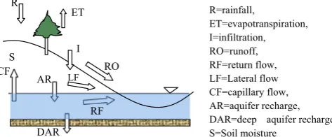
the USDA Conservation Effects Assessment Project (CEAP).Gosain et al. (2006)modeled twelve large river catchments in India with the purpose of quantifying the climate change impact on hydrol-ogy.Schuol et al. (2008)simulated hydrology of the entire Africa with SWAT in a single project and calculated water resources at a subbasin spatial resolution and monthly time intervals. Faramarzi et al. (2009) simulated hydrology and crop yield for Iran with SWAT. In a subsequent work,Faramarzi et al. (2013)used the African model to study the impact of climate change in Africa. R=rainfall, ET=evapotranspiration, I=infiltration, RO=runoff, RF=return flow, LF=Lateral flow CF=capillary flow, AR=aquifer recharge, DAR=deep aquifer recharge S=Soil moisture S R ET I RO RF AR CF DAR LF
Fig. 1.Schematic illustration of the conceptual water balance model in SWAT.
Table 1
Data description and sources used in the European SWAT project.
Data type Resolution Source
Digital Elevation (DEM)
90 m aggregated to 700 m
Shuttle Radar Topography Mission (SRTM)http://www2.jpl.nasa.gov/ srtm/
Soil 5 km FAO–UNESCO global soil map
http://www.fao.org/nr/land/soils/ digital-soil-map-of-the-world/en/
Landuse – 300 m – GlobCover European Space Agencyhttp://due.esrin.esa. int/globcover/
– 1000 m – Global Landuse/Land Cover Characterization USGS
http://landcover.usgs.gov/glcc/
– 500 m – MODIS land cover http://modis-land.gsfc.nasa.gov/
– 300 m – GlobCorine provided by European Space Agencyhttp:// www.esa.int/About_Us/ESRIN/ Express_map_delivery_from_ space
River network dataset
ffi62 km2avg. size
catchment
European catchments and Rivers network System (Ecrins)http:// projects.eionet.europa.eu/ecrins
Climate – Observed – National Climate Data Center (NCDC),http://www.ncdc. noaa.gov/
– 0.25°grid – European Climate Assessment Dataset (ECAD),http://www.ecad. eu/
– 0.5°grid – Climate Research Unit (CRU),
http://www.cru.uea.ac.uk/
– 1°grid – Climate Data Guide (NCAR),
https://climatedataguide.ucar. edu/
River discharge 326 stations Global Runoff Data Center (GRDC)
http://www.bafg.de/GRDC/EN/ Home/homepage_node.html
Nitrate loads 34 stations ICPDRhttp://en.wikipedia.org/ wiki/International_
Commission_for_the_Protection_ of_the_Danube_River
Crop yield Wheat, maize, barley
McGill Univesityhttp://www. geog.mcgill.ca/landuse/pub/Data/ 175crops2000/NetCDF/
FAOSTA – Country-based average crop yield Agricultural management and water resources Planting, harvesting, fertilization-blue water FAOSTAThttp://faostat.fao.org/ site/339/default.aspx
– AQUASTAT, FAOhttp:// www.fao.org/nr/water/aquastat/ water_res/index.stm
Population Eurostathttp://epp.eurostat.ec. europa.eu/portal/page/portal/ population/introduction
Population growth rate
World Bankhttp://
data.worldbank.org/indicator/SP. POP.GROW
Point source pollution
SWAT is recognized by the U.S. Environmental Protection Agency (EPA) and has been incorporated into the EPA’s BASINS (Better Assessment Science Integrating Point and Non-point Sources). The larger capacity of ArcGIS (version 9.3 and higher) now allows building finer resolution large-scale models, which could be calibrated using powerful parallel processing (Rouholahnejad et al., 2012) and grid computations (Gorgan et al., 2012), allowing proper uncertainty analysis.
SWAT-CUP (Calibration and Uncertainty Procedures) (Abbaspour et al., 2007) is a standalone program developed for
calibration of SWAT. The program contains five different calibra-tion procedures and includes funccalibra-tionalities for validacalibra-tion and sensitivity analysis as well as visualization of the area of study using Bing Map. With this feature, the subbasins, simulated rivers, and outlet, rainfall, and temperature stations can be visualized on the Bing map. In the current work we used the pro-gram SUFI-2 (Abbaspour et al., 2004; Abbaspour et al., 2007) for model calibration and uncertainty analysis. For time-consuming large-scale models, SUFI-2 was found to be quite efficient (Yang et al., 2008).
Against this background, the goal of this work is to use SWAT to build a hydrological model of Europe at subbasin level and monthly time intervals. The key objectives of this work are: (i) to incorporate agricultural management and crop yield to the hydrological model for a more accurate calculation of evapotranspiration, (ii) to add water quality to the model by adding point sources and diffuse sources of nitrogen to investigate the nitrate leaching into the groundwater, (iii) to quantify spatial and temporal variations in water availability at European Continent scale. In particular, components such as blue water (water yield plus deep aquifer recharge), green water flow (evapotranspiration), green water storage (soil moisture), and nitrate concentration of groundwater recharge are quantified. The model estimations at the subbasin level are then aggregated to country and river basin levels for comparison with other studies. The results from this study provide a consistent information package on the quantity and quality of water resources on tem-poral and spatial dimensions, and on internal renewable water resources for individual countries across Europe. A calibrated model at this scale can be used for various analyses such as cross-boundary water analysis, assessment of nitrate loads gener-ated in various countries; quantification of the nitrate input into various lakes, sees, and ocean; highlighting the sources of contami-nant generation; and finally studying the impact of climate and landuse change on the continent’s water resources.
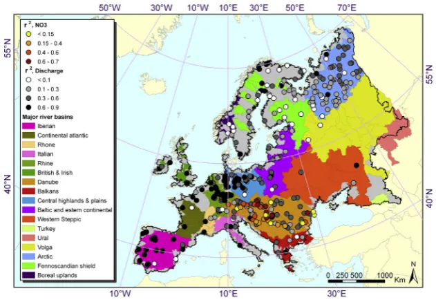
Fig. 2.Map of the modeled area showing the location of measured discharge and
nitrate stations as well climate CRU grid points.
Fig. 3.Illustration of the visualization module in SWAT-CUP. This allows gathering information from the site that helps with model parameterization and parameter range
identification. Figure (a) shows positioning of an outlet on Viar river instead of on the main Rio Guadalquivir in Spain; figure (b) shows position of an outlet downstream of a dam on Inn River near Munich, Germany; figure (c) shows a complex river geometry on Pechora River near Golubovo in Russia; figure (d) shows an outlet governed by glacier melt near Martigny in Switzerland. These features could explain some of the discrepancies between simulation and observed results if parameterized incorrectly. The red– green symbol indicates location of the outlet. (For interpretation of the references to color in this figure legend, the reader is referred to the web version of this article.)
2. Material and methods
2.1. The large-scale hydrological simulator SWAT
The SWAT program is a comprehensive, semi-distributed, con-tinuous-time, processed-based model (Arnold et al., 2012; Neitsch et al., 2005; Gassman et al., 2007). The program can be used to build
models to evaluate the effects of alternative management decisions on water resources and non-point source pollution in large river basins. The hydrological component of SWAT (Fig. 1) allows explicit calculation of different water balance components, and subsequently water resources (e.g., blue and green waters) at a subbasin level.
In SWAT, a watershed is divided into multiple subbasins, which are then further subdivided into hydrologic response units (HRUs)
Table 2
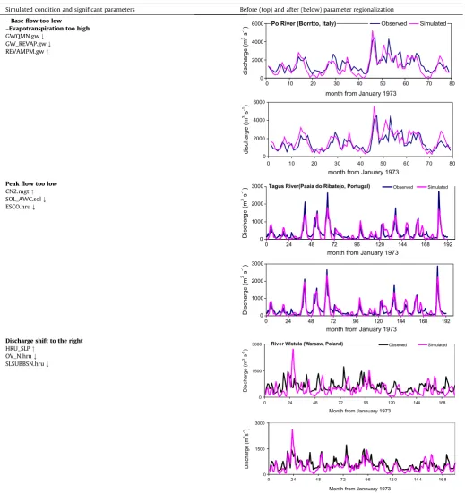
Rules for parameter regionalization."indicates parameter should increase,;indicates parameter should decrease. (For more detail see SWAT calibration validation literature
http://swat.tamu.edu/publications/calibrationvalidation-publications/).
Simulated condition and significant parameters Before (top) and after (below) parameter regionalization
–Base flow too low Po River (Borrtto, Italy)
0 2000 4000 6000
0 10 20 30 40 50 60 70 80
month from January 1973
discharge (m
3 s -1)
Observed Simulated
0 2000 4000 6000
0 10 20 30 40 50 60 70 80
month from January 1973
discharge (m
3 s -1)
–Evapotranspiration too high
GWQMN.gw;
GW_REVAP.gw;
REVAMPM.gw"
Peak flow too low Tagus River(Paaia do Ribatejo, Portugal)
0 1000 2000 3000
0 24 48 72 96 120 144 168 192
month from January 1973
Discharge (m
3 s -1 )
Observed Simulated
0 1000 2000 3000
0 24 48 72 96 120 144 168 192
Discharge (m
3 s -1 )
month from January 1973 CN2.mgt"
SOL_AWC.sol;
ESCO.hru;
Discharge shift to the right River Wistula (Warsaw, Poland)
0 1500 3000
0 24 48 72 96 120 144 168
D
is
c
har
ge (
m
3 s -1)
Observed Simulated
0 1500 3000
0 2 4 4 8 7 2 9 6 12 0 14 4 16 8
Discharge (m
3s
-1)
Month from Jannuary 1973
Month from Jannuary 1973
HRU_SLP"
OV_N.hru;
that consist of unique landuse, management, topographical, and soil characteristics. Simulation of watershed hydrology is done in the land phase, which controls the amount of water, sediment, nutrient, and pesticide loadings to the main channel in each sub-basin, and in the routing phase, which is the movement of water, sediments, etc., through the streams of the subbasins to the outlets. The hydrological cycle is climate driven and provides moisture and energy inputs, such as daily precipitation, maximum/mini-mum air temperature, solar radiation, wind speed, and relative humidity that control the water balance. Snow is computed when temperatures are below freezing, and soil temperature is com-puted because it impacts water movement and the decay rate of residue in the soil. Hydrologic processes simulated by SWAT include canopy storage, surface runoff, and infiltration. In the soil the processes include lateral flow from the soil, return flow from shallow aquifers, and tile drainage, which transfer water to the river; shallow aquifer recharge, and capillary rise from shallow aquifer into the root zone, and finally deep aquifer recharge, which removes water from the system. Other processes include moisture redistribution in the soil profile, and evapotranspiration. Optionally, pumping, pond storages, and reservoir operations could also be considered. The water balance for reservoirs includes inflow, outflow, rainfall on the surface, evaporation, seepage from the reservoir bottom, and diversions.
Addressing vegetation growth is essential in a hydrological model as evapotranspiration is an important component of water balance, and management operations such as irrigation (Faramarzi et al., 2009) and fertilization have a large impact on hydrology and water quality, respectively. SWAT uses a single plant growth model to simulate growth and yield of all types of
land covers and differentiates between annual and perennial plants.
In addition, SWAT simulates the movement and transformation of several forms of nitrogen and phosphorus, pesticides, and sedi-ment in the watershed. SWAT allows users to define managesedi-ment practices taking place in every HRU. Once the loadings of water, sediment, nutrients, and pesticides from the land phase to the main channel have been determined, the loads are routed through the streams and reservoirs within the watershed. More details on the SWAT can be found in the theoretical documentation (http:// swatmodel.tamu.edu) and inArnold et al. (1998).
2.2. Databases
The model for the continent of Europe was constructed using, for most parts, freely available data (Table 1). These data were complemented by additional sources provided by project partners on climate and agricultural management.
2.3. Model setup
The ArcSWAT 2009 interface is used to setup and parameterize the model. On the basis of DEM and the stream network, a thresh-old drainage area of 5000 km2was chosen to discretize the conti-nent into 8592 subbasins, which were further subdivided into 60,012 HRUs based on soil, landuse, and slope. Each HRU is thought to be a uniform unit where water balance calculations are made. The entire simulation period is from 1970 to 2006. As each station has data for different years, we used about two-third of the data for calibration and the remaining for validation. The first 3 years are
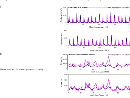
Table 2(continued)
Simulated condition and significant parameters Before (top) and after (below) parameter regionalization
–Base flow too high River Usa (Chum, Russia)
0 2000 4000
0 50 100 150 200
D
is
c
har
ge (
m
3s -1)
Observed Simulated
0 2000 4000
0 50 100 150 200
D
is
c
har
ge (
m
3s -1)
Month from January 1973
Month from January 1973
–Peaks too low
CN2.mgt"
SOL_AWC.sol;
ESCO.hru;
GWQMN.gw"
GW_REVAP.gw"
REVAMPM.gw;
Nitrate load too high River Danube (Edramsberg, Austria)
0 20000 40000 60000
0 20 40 60 80 100
Observed Simulated
0 20000 40000 60000
0 20 40 60 80 100
Nitrate (tn)
Nitrate (tn)
month from August 1996 month from August 1996
SHALLST_N.gw;
RCN.bsn;
NPERO.bsn;
CMN.bsn;
SOL_NO3.chm;
FRT_SURFACE.mgt;(in our case also decreasing parameterain Eq.(1))
used as equilibration period to mitigate the initial conditions and were excluded from the analysis. This large project was built on a laptop with a 64 bit operating system, 4 CPUs, 8 GB of RAM and 2.7 GHz processors. It took about 12 h for a single SWAT run of 37 years. Initial runs were performed with the parallel process-ing routine linked to SUFI-2 (Rouholahnejad et al., 2012). Final runs were performed using the server-based network cluster gSWAT (Gorgan, et al., 2012; Mihon, et al., 2013).
In general, the state of freely available river discharge measure-ments in terms of water quantity and quality, and crop yield data is relatively poor in Europe. A total of 326 discharge stations and only 34 stations with nitrate data were found reliable enough to be used in model calibration/validation process (Fig. 2). Majority of the measured nitrate stations were on the Danube River. Furthermore, much correction needed to be made to the river data as many broken links caused wrong flow directions, and many cor-rections were also made to the coordinates of the measured dis-charge stations. Lack of precision in the coordinates causes ArcSWAT to place the observed outlets on the wrong river, causing a major calibration problem. The visualization option of SWAT-CUP, using the Bing map, is of paramount help in detecting these problems and other abnormalities (Fig. 3).
Five elevation bands were used in the model to adjust the tem-perature and rainfall based on subbasin elevation variation. As detailed operational information on lakes and reservoirs were lack-ing, we did not use any outlets that were influenced directly by reservoirs.
Point sources of pollution were assigned to each subbasin based on the population percentage connected to sewage treatment plant (Eurostat 2000–2009). This percentage was above 80% in
approximately half of the European Union countries for which data were available. As the data was not available for all countries and all years from 1970 to 2006, we made a few assumptions. For example, Moldova, Ukraine, Russia, Belarus, and Georgia were assumed to have the same rates as Bulgaria. Serbia, Bosnia, Montenegro was assumed to be in the same situation as Slovenia. Also, point source discharges 1970–2000 were assumed to be constant and equal to year 2000. In terms of treatment levels, tertiary wastewater treatment was most common in Germany, Austria and Italy where at least four in every five persons were connected to this type of wastewater treatment. In contrast, not more than 1% of the population was connected to tertiary wastewater treatment in Romania and Bulgaria. We assumed the treatment efficiency to be 80% in all cases. Furthermore, the efflu-ent from 20% of the pollution was assumed to be untreated wastewater and directly loaded into surface waters.
The regional population was calculated based on the population map in the year 2005 (CIESIN, 2005) and extrapolated to other years based on the national population growth rate provided by World Bank.Zessner and Lindtner (2005)investigated the emis-sions of nutrient from municipal point sources based on detailed evaluation of data from 76 municipal wastewater treatment plants and calculation of discharge of nitrogen (N) from households into wastewater in Austria. The results of this investigation show that the average value of nitrogen load is 8.8 gN/Peday for municipal
wastewater (contributions from households and industry). Population equivalentPeaccounts for industrial releases. Nitrate
loading to rivers was calculated as:
LN¼
a
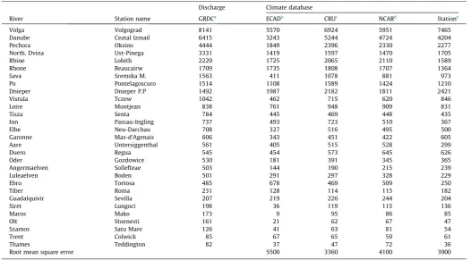
iPeIN½ð1SrateÞ þ ð1TeffÞSrate; ð1Þ Table 3Simulated mean annual river discharges (m3s1) for a selection of European rivers based on four different climate datasets.
Discharge Climate database
River Station name GRDCa ECADb CRUc NCARd Statione
Volga Volgograd 8141 5570 6924 5951 7465
Danube Ceatal Izmail 6415 3243 5244 4724 4204
Pechora Oksino 4444 1849 2396 2330 2277
North. Dvina Ust-Pinega 3331 1419 1597 1470 1705
Rhine Lobith 2229 1725 2065 2110 1589
Rhone Beaucairw 1709 1735 1808 1707 1364
Sava Sremska M. 1563 411 1078 881 973
Po Pontelagoscuro 1514 1108 1589 1424 1210
Dnieper Dnieper P.P 1492 1987 2182 1811 2421
Vistula Tczew 1042 462 715 620 846
Loire Montjean 838 761 948 909 831
Tisza Senta 784 445 469 448 435
Inn Passau-Ingling 737 493 723 510 367
Elbe Neu-Darchau 708 327 516 495 500
Garonne Mas-d’Agenais 606 343 451 422 605
Aare Untersiggenthal 561 405 515 528 299
Duero Regua 545 454 573 645 626
Oder Gozdowice 530 181 391 345 365
Angermaelven Sollefteae 503 144 190 215 239
Luleaelven Boden 501 291 297 328 229
Ebro Tortosa 485 678 469 509 250
Tiber Roma 231 128 114 115 182
Guadalquivir Sevilla 207 219 226 244 204
Siret Lungoci 198 36 119 115 136
Maros Mako 173 9 95 86 85
Olt Stoenesti 161 21 62 67 47
Szamos Satu Mare 126 41 63 81 54
Trent Colwick 85 67 65 59 61
Thames Teddington 82 37 47 72 36
Root mean square error 5500 3360 4100 3900
aThe GRDC values are the observed annual average river discharges (m3s1). b ECAD, European Climate Assessment Dataset.
c CRU, Climate Research Unit. d NCAR, Climate Data Guide.
where LN is the nitrate loading to river from the subbasins
con-tributing to outleti(g day1),
ai
is a correction factor we added to adjust the quantity of input load based on the long-term average nitrate load of the river at outleti,INis the average input of nitrogenfrom household to wastewater (g NPe1day1),Srateis the
percent-age of the population connected to any kind of sewpercent-age treatment, andTeffis the wastewater treatment efficiency assumed to be 0.8.
Three major crops, maize, wheat and barley, were considered in this study. These crops were allocated to ‘‘agricultural land’’ in lan-duse maps and their planting areas in each subbasin proportioned
to their planted areas in each country as indicated in MIRCA2000 report (Portmann et al., 2010). Irrigated and rainfed cropping areas were differentiated based on the MIRCA2000 report at a spatial resolution of 5 arc min. Crop yield for model calibration was obtained fromMonfreda et al. (2008)at 5 arc minute resolution and from FAOSTAT at country level.
Twenty-five different management plans were designed across Europe based on the crop type, planting and harvest dates, winter or summer crops, irrigated or rain-fed applications. Automatic fer-tilization scheduling was employed based on plant nutrient deficit
Fig. 4.Overall modeling results at observed discharge and nitrate stations.r2is used as an index showing the goodness of fit.
Discharge
Nitrate
Fig. 5.P-factorversusR-factor.P-factoris the percentage of observed data bracketed by the 95PPU.R-factoris the width of the 95PPU band. A working value of >0.7 forP-factor
and <1.5 forR-factoris recommended.
and the annual maximum application amount was set to 300 kg N ha1. Elemental nitrogen and elemental phosphors were selected as the main fertilizer. A few parameters were fitted to match the long-term (1973–2006) average country yields reported by FAO. These included: total heat units for crops to reach maturity (HEAT_UNITS); harvest index (HI_TARG) and biomass target (BIO_TARG), which allow control of biomass production by the plant every year; nitrogen stress factor (AUTO_NSTRS), which ensures that there is almost no reduction of plant growth due to nutrient stress; application efficiency (AUTO_EFF), which allows the model to apply fertilizer to meet harvest removal plus an extra amount to make up for nitrogen losses due to surface runoff/leach-ing; and fraction of fertilizer applied to top 10 mm of soil (AFERT_SURFACE), where the remaining fertilizer is applied to the first soil layer. Irrigation was based on plant-water-stress auto-matic scheduling, and withdrawn from outside sources so that the model will add water to the soil until its field capacity. We fitted water stress threshold (Auto_WSTRS), which triggers irrigation, and irrigation efficiency (IRR_EFF). Remaining crop parameters and parameters for non-crop land covers originated from SWAT default database (Neitsch et al., 2005). Parameters sensitive to crop model outputs, such as heat units, were subsequently calibrated to the local conditions.
In this study, potential evapotranspiration (PET) was estimated using the Hargreaves method (Hargreaves et al., 1985) while actual evapotranspiration (ET) was estimated based on Ritchie (Ritchie, 1972). The daily value of leaf area index was used to partition between evaporation and transpiration.
2.4. Calibration, parameterization, and uncertainty analysis
The SUFI-2 algorithm (Abbaspour et al., 2004, 2007) in the SWAT-CUP software package (Abbaspour, 2011) was used for model calibration, validation, sensitivity, and uncertainty analysis. This algorithm maps all uncertainties (parameter, conceptual model, input, etc.) on the parameters (expressed as uniform
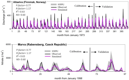
distributions or ranges) and tries to capture most of the measured data within the 95% prediction uncertainty (95PPU) of the model in an iterative process. The 95PPU is calculated at the 2.5% and 97.5% levels of the cumulative distribution of an output variable obtained through Latin hypercube sampling. For the goodness of fit, as we are comparing two bands (the 95PPU for model simulation and the band representing measured data plus its error), the first author coined two indices referred to as ‘‘P-factor’’ and ‘‘R-factor’’ (Abbaspour et al., 2004). TheP-factoris the fraction of measured data (plus its error) bracketed by the 95PPU band and varies from 0 to 1, where 1 indicates 100% bracketing of the measured data within model prediction uncertainty (i.e., a perfect model sim-ulation considering the uncertainty). The quantity (1P-factor) could hence be referred to as the model error. For discharge, we recommend a value of >0.7 or 0.75 to be adequate. This of course depends on the scale of the project and adequacy of the input and calibrating data. TheR-factoron the other hand is the ratio of the average width of the 95PPU band and the standard deviation of the measured variable. A value of <1.5, again depending on the situation, would be desirable for this index (Abbaspour et al., 2004, 2007). These two indices are used to judge the strength of the calibration and validation. A largerP-factor can be achieved at the expense of a largerR-factor. Hence, often a balance must be reached between the two. In the final iteration, where accept-able values of R-factor and P-factor are reached, the parameter ranges are taken as the calibrated parameters. SUFI-2 allows usage of ten different objective functions such asr2, Nash-Sutcliff (NS), and mean square error (MSE). In this study we usedbr2 for dis-charge and nitrate loads. The efficiency criterion was defined as (Krause et al., 2005):
/¼ jbjr
2 for jbj 1
jbj1r2 for jbj
>1
(
; ð2Þ
wherer2is the coefficient of determination andbis the slope of the regression line between the measured and simulated variables. The Altaelva (Finnmak, Norway)
0 400 800
1 25 49 73 97 121 145 169 193 217 241 265 289 313 337 361 385
month from January 1973
Discharge (m
3 s -1 )
Marva (Rabensberg, Czeck Republic)
0 3000 6000
1 25 49 73 97
month from January 1998
Nitrate (t ha
-1 )
P-factor= 0.77
R-factor= 1.17
R2= 0.63 NS= 0.60
95PPU Observed Simulated
Calibration Validation
P-factor= 0.77
R-factor= 1.17
R2= 0.63 NS= 0.60
95PPU Observed Simulated
Validation Calibration
Fig. 6.Illustration of full SWAT-CUP output showing the observed, the best simulation, and the 95% prediction uncertainty (95PPU).P-factoris the percentage of observations
objective function containing two variables (e.g., river discharge and nitrate load) at multiple sites was formulated as:
H
¼ 1wv1þwv2
wv1
Pn1 i¼1wi
X n1
i¼1
wi/iþ wv2
Pn2 i¼1wi
X n2
i¼1
wi/i
" #
; ð3Þ
wherewv1andwv2are weights of the two variables,n1andn2are the number of discharge and nitrate stations, respectively, andwi’s are
the weights of variables at each station. The function/, and conse-quentlyHvary between 0 and 1. In this form, the objective function, unlike, for example, NS, which may range from1 to 1, is not 0
1500 3000
0 24 48 72 96 120 144 168 192 216 240 264
Discharge (m
3s -1)
Month from January 1973
Usa (Chum, Russia) Observed
0 15000 30000
0 24 48 72 96 120 144 168 192 216 240 264
Discharge (m
3s -1)
Month from May 1980
Pechora (Golubov, Russia)
0 400 800
0 24 48 72 96 120 144 168 192
Discharge (m
3s -1)
Month from January 1973
Vishera (Bogorodsk, Russia)
0 5000 10000
0 24 48 72 96 120 144 168 192 216 240 264 288 312
D
is
c
h
ar
ge (
m
3s -1)
Month from January 1973
Vychegda (Fedyakovo, Russia)
0 300 600
0 24 48 72 96 120 144 168 192 216 240 264 288 312 336 360 384
Discharge (m
3s -1)
Month from January 1973
Kautokeino (Masi, Norway)
R
2=0.29, NS=0.25
P-factor=0.67;
R-factor
=0.63
a
R
2=0.63, NS=0.53
P-factor=0.39;
R-factor=0.54
b
R
2=0.21, NS=0.91
P-factor=0.53;
R- factor
=0.76
c
R
2=0.56, NS=-0.66
P-factor
=0.63;
R-factor
=0.99
d
R
2=0.34, NS=0.26
P-factor=0.76; R-factor=0.97
e
R
2=0.61, NS=0.54
P-factor
=0.66;
R-factor
=0.95
f
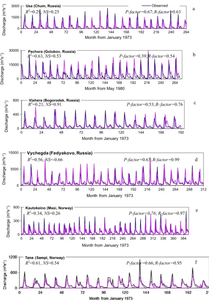
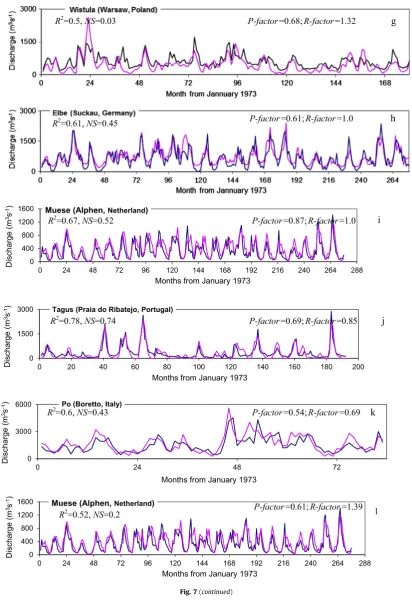
Fig. 7.Illustration of model results for some major rivers across Europe. The figures covers both calibration and validation periods. The statisticsr2,NS, andaare for both
periods,P-factorandR-factorare for validation period only.
dominated by any one or a few very badly simulated stations. Weights in Eq.(3)become critical if an objective function such as mean square error is used, but because of usingbr2they do not make a significant difference to model calibration results. For this reason we set all weights to 1. For crop yield, which was calibrated after an initial calibration of the model for discharge and nitrate, we used mean square errors for each crop as the objective function:
/3¼
1 n3
Xn3
i¼1
Yoi Y s i 2
; ð4Þ
wheren3is the number of sites with wheat, barley, and corn yield data,Yo(t ha1) is the observed yield, and
Ys(t ha1) is the simu-lated yield.
0 400 800 1200 1600
0 24 48 72 96 120 144 168 192 216 240 264 288
Discharge (m
3s -1)
Months from January 1973
Muese (Alphen, Netherland)
0 1500 3000
0 20 40 60 80 100 120 140 160 180 200
Discharge (m
3s -1)
Months from January 1973
Tagus (Praia do Ribatejo, Portugal)
0 3000 6000
0 24 48 72
Discharge (m
3s -1)
Months from January 1973
Po (Boretto, Italy)
0 400 800 1200 1600
0 24 48 72 96 120 144 168 192 216 240 264 288
Discharge (m
3s -1)
Months from January 1973
Muese (Alphen, Netherland)
R
2=0.5, NS=0.03
P-factor
=0.68;
R-factor
=1.32
g
R
2=0.61, NS=0.45
P-factor
=0.61;
R-factor
=1.0
h
R
2=0.67, NS=0.52
P-factor
=0.87;
R-factor
=1.0
i
R
2=0.78, NS=0.74
P-factor
=0.69;
R-factor
=0.85
j
R
2=0.6, NS=0.43
P-factor
=0.54;
R-factor
=0.69
k
R
2=0.52, NS=0.2
P-factor
=0.61;
R-factor
=1.39
l
Danube (Drobeta-Turnu Severin, Romania)
0 30000 60000 90000
0 24 48 72 96
Month from January 1997
Nitrate (tha
-1)
Observed Simulated
Danube (Vacareni, Romania)
0 40000 80000 120000
0 24 48 72 96
Month from January 1997
Nitrate (t ha
-1
)
Danube (Wien-Nussdorf, Austria)
0 20000 40000
0 24 48 72 96
Month from January 1998
Nitrate (t ha
-1)
Danube (Ottenheim, Austria)
0 10000 20000 30000
0 24 48 72 96 120
Months from January 1996
Nitrate (t ha
-1)
Danube (Günzburg, Germany)
0 3000 6000
0 24 48 72 96 120
Month from January 1996
Nitrate (t ha
-1)
Danube (Bratislava, Slovakia)
0 15000 30000 45000
0 24 48 72
Months from January 1998
Nitrate (t ha
-1)
Danube (Szobe, Hungary)
0 20000 40000 60000
0 24 48 72 96
Month from January 1998
Nitrate (t ha
-1
)
R
2=0.28,
NS
=0.12,
α
=0.2
P-factor
=0.63;
R-factor
=1.5
a
R
2=0.62,
NS
=0.57,
α
=0.22
P-factor
=0.65;
R-factor
=1.3
b
R
2=0.54,
NS
=0.45,
α
=0.52
P-factor
=0.7;
R-factor
=1.6
c
R
2=0.58,
NS
=0.39,
α
=0.5
P-factor
=0.64;
R-factor
=1.6
d
R
2=0.58,
NS
=-0.39,
α
=
0.63
P-factor
=0.61;
R-factor
=1.9
e
R
2=0.64,
NS
=0.51,
α
=0.53
P-factor
=0.73;
R-factor
=1.7
f
R
2=0.65,
NS
=0.61,
α
=0.42
P-factor
=0.72;
R-factor
=1.6
g
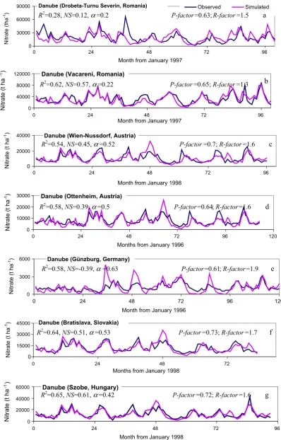
Fig. 8.Examples of model simulation results for nitrate loads on different locations on the Danube River and on other rivers, which are mostly tributaries of Danube. The
Morava (Rabensburg, Czeck Republic)
0 1500 3000
0 24 48 72 96
Month from January 1998
Nitrate (t ha
-1 ) Observed Simulated
Sajo (Sajopuspoki, Hungary)
0 400 800
0 24 48 72 96
Month from January 1998
Nitrate (t ha
-1
)
Salzach (Burghausen, Germany)
0 800 1600
0 24 48 72 96 120
Month from January 1996
Nitrate (t ha
-1)
Tisza (Ruski Krstur, Hungary)
0 6000 12000 18000
0 24 48 72 96
Month from January 1998
Nitrate (t ha
-1 )
Drava (Donja Dubrava, Croatia)
0 1000 2000 3000
0 24 48 72 96 120
Month from Feruary 1996
Nitarte (t ha
-1)
Sava (Jesenice, Slovania)
0 2000 4000
0 24 48 72 96 120
Month from February 1996
Nitrate (t ha
-1)
Sava (Bosanska Gradiska, Croatia)
0 5000 10000
0 12 24 36
Month from January 2003
Nitrate (t ha
-1)
R
2=0.62,
NS
=0.59,
α
=0.6
P-factor
=0.8;
R-factor
= 1.32
h
R
2=0.2,
NS
=-0.04,
α
=0.63
P-factor
=0.72;
R-factor
=1.5
i
R
2=0.31,
NS
=-0.36,
α
=0.28
P-factor
=0.8;
R-factor
=2.4
i
R
2=0.61,
NS
=0.48,
α
=0.2
P-factor
=0.75;
R-factor
=1.6
i
R
2=0.46,
NS
=0.33,
α
=0.2
P-factor
=0.6;
R-factor
=1.9
j
R
2=0.42,
NS
=0.2,
α
=0.3
P-factor
=0.5;
R-factor
=1.4
k
R
2=0.38,
NS
=0.16,
α
=2.2
P-factor
=0.72;
R-factor
=1.5
l
2.4.1. Calibration protocol for large-scale distributed models
To calibrate the model we used the following general approach:
(1) Build the model with ArcSWAT using the best parameter estimates based on the available data, literature, and ana-lyst’s expertise. There is always more than one data set (e.g., soil, landuse, climate, etc.) available for a region. For Europe we were in possession of four different landuse maps, two different soil maps, and four different sets of cli-mate data (Table 1). Hence, initially several models were built and ran without any calibration (referred as the default model) with different databases. The model results were compared with observations (discharge and nitrate) and the best overall performing database was selected for fur-ther analysis. It should be noted that the performance of the default model should not be too drastically different from the measurement. If so, often calibration can be of little help.
(2) Use the best default model to calibrate. Based on the perfor-mance of the default model at each outlet station, relevant parameters in the upstream subbasins are parameterized using the guidelines summarized inTable 2. This procedure results in regionalization of the parameters.
(3) Based on parameters identified in step 2 and one-at-a-time sensitivity analysis, initial ranges are assigned to parameters of significance. Experience and hydrological knowledge of the analyst is also of great asset in defining parameter ranges. In addition to the initial ranges, user-defined abso-lute parameter ranges are also defined for every SWAT parameter in SWAT-CUP where parameters are not allowed to be outside of this range.
(4) Once the model is parameterized and the ranges are assigned, the model is run some 300–1000 times, depending on the number of parameters, speed of the model execution, and the system capabilities. Great time saving could be achieved by using the parallel processing option of SWAT-CUP (Rouholahnejad et al., 2012).
(5) After all simulations are completed; the post processing option in SWAT-CUP calculates the objective function and the 95PPU for all observed variables in the objective func-tion. New parameter ranges are suggested by the program
for another iteration, which modifies the previous ranges focusing on the best parameter set of the current iteration (Abbaspour et al., 2004, 2007).
(6) The suggested new parameter ranges could be modifies by the user usingTable 2and one-at-a-time sensitivity analysis again. Another iteration is then performed. The procedure continues until satisfactory results are reached (in terms of the P-factor andR-factor) or no further improvements are seen in the objective function. Normally, three to five itera-tions are sufficient for satisfactory results. More detailed information could be found in Abbaspour et al. (2004, 2007)andRouholahnejad et al. (2012).
3. Results
3.1. Calibration/validation of discharge
In the preliminary analyses we tested different landuse and cli-mate databases and selected Modis landuse map and CRU’s 0.5° global climate database. The selection was based on a comparison of measured discharges of major rivers against default model sim-ulations (Table 3). We chose the CRU climate database because it had the smallest overall error. The difference from different lan-duses however was not very significant. To compare the model results here with other past or future works, we should keep in mind the inputs used to develop this model as using, for example, a different climate database, would result in different outputs.
The overall performance of the model in terms ofr2has quiet satisfactory results for the European model (Fig. 4). It should be kept in mind that all 326 discharge outlets and 34 nitrate outlets were parameterized and optimized simultaneously. This results in an overall good simulation, and may results in some individual outlets to be poorly simulated. A more local simulation with a smarter algorithm that could account for nested outlets would certainly result in a better overall simulation. A graph ofP-factor
versus R-factor (Fig. 5) shows that a large number of the 326 outlets fall in desirable regions of the two indices. A few outlets were located downstream of dams. These outlets would of course not be well simulated by SWAT in any way as their flow regimes are entirely controlled by the operation of the dam or reservoir. Hence, we plotted these factors after removing those outlets, which had quite large R-factor. For nitrate, the uncertainties, as indicated by theR-factorare generally larger. As SUFI-2 is iterative, each iteration results in a reduction of parameter uncertainties causing a narrower 95PPU band, which subsequently results in a smaller P-factor. Hence, a balance must be struck between the two indices.
In general, model uncertainties are due to: (i) conceptual sim-plifications (e.g., SCS curve number method for flow partitioning), (ii) processes occurring in the watershed but not included in the program (e.g., wind erosion, wetland processes), (iii) processes that are included in the program, but their occurrences in the water-shed are unknown to the modeler or unaccountable because of data limitation (e.g., dams and reservoirs, water transfers, farm management affecting water quality), and (iv) input data quality. In large watershed applications one expects to have all these forms of uncertainties, which explains some of the large prediction errors. In this study, outlets on rivers with small flows showed par-ticularly large uncertainties.
In the following we describe some details of the important river basins of Europe (colored1inFig. 4). The characteristics of major
riv-ers and the model performances are assessed for both discharge and
Fig. 9.Map of runoff ratio (runoff/rainfall) providing an indication of erosion
potential.
1For interpretation of color in Fig. 4, the reader is referred to the web version of
this article.
nitrate. SWAT-CUP produces output results at each station as 95PPU as well as showing the best fit (e.g., the simulation run with the best objective function value) (Fig. 6), but for simplicity and clarity of pre-sentation we only show the calibration/validation results for the best simulation as a continuous graph (Figs. 7and8) and report the over-all statistics.
The river discharges in the northeast corner of Europe in Russia are governed by snow melts. They are frozen in winter and active in the spring and summer. This is evident from the regular peaks in the spring and near zero discharges in winter months. Examples from rivers Usa (length = 565 km, Basin area = 93,600 km2), Pechora (1800 km, 322,000 km2), and Vishera (415 km, 31,200 km2) (Fig. 7a–c) are characterized with freezing around October–November, and staying frozen until the spring thaw in April–May. This region was calibrated using among other parame-ters SNOEB (initial snow water content), SFTMP (snowfall tempera-ture), SMTMP (snow melt base temperatempera-ture), SMFMX (melt factor on June 21st), and SMFMN (melt factor on December 21st), as well as by increasing the CRU rainfall throughout the year by about 20%. Increasing the rainfall was important to catch the peaks of spring and summer discharges. SWAT accumulates the rainfall during fall and winter as snow, and then melts the snow in spring and sum-mer. The larger discrepancy in the recession dynamics between
observed and simulated discharges in the Pechora River (Fig. 7b) is due to the complex branching of this main river before the point of measurement (Fig. 3c). Given the complexity of the system, it is surprising that the model can still simulate the discharge at this location with such accuracy (r2= 0.63,NSE= 0.53) albeit with small
P-factor(0.39).
Further west still in the European part of Russia, is the Vychegda River (1100 km, 120,000 km2) (Fig. 7d), a tributary to the Northern Dvina, with a large average discharge rate of over 1000 m3s1. Simulation of this navigable river, although visually very good, suffers from a small lag in the simulation, which could not be corrected by the parameters listed inTable 2. This could have been caused by a small shift in the CRU rainfall governing this outlet in SWAT.
In the far north of Europe is Kautokeino River (Fig. 7e) in Norway (240 km, 7400 km2). This river drains into Alta river and then to the Norwegian Sea and is fed by a complex system of lakes, peatlands, and tributaries. The result shows relatively good sim-ulation of the river discharge dynamics (r2= 0.34).
The Tana River (Fig. 7f) in northern Scandinavia (361 km, 16,000 km2) flows in pristine condition through Norway and the Lapland region of Finland. This river is very well simulated (r2= 0.61,NS= 0.54) with a rather largeP-factor(0.66).
0.0 2.0 4.0 6.0 8.0 10.0
Albania Austria Belarus Belgium Bosnia Bulgaria Croatia czeck Denmark Finland France Germany Greece Hungary Irland Italy Latvia
Lithuania
Netherland
Norway Poland
Portugal Romania Russia Slovakia Slovania
Spain
Sweeden
Switzerland
Ukrain
UK
Wheat yield (tn ha
-1 )
95PPU FAO McGill
0.0 2.0 4.0 6.0 8.0 10.0
Albania Austria Belarus Belgium Bosnia Bulgaria Croatia czeck Denmark Finland France Germany Greece Hungary Irland Italy Latvia
Lithuania
Netherland
Norway Poland
Portugal Romania Russia Slovakia Slovania
Spain
Sweeden
Switzerland
Ukrain
UK
Barley yield (tn ha
-1)
95PPU FAO
0.0 2.0 4.0 6.0 8.0 10.0 12.0
Albania Austria Belarus Belgium Bosnia
Bulgaria Croatia czeck France Germany Greece Hungary
Italy
Lithuania
Netherland
Poland
Portugal Romania Russia Slovakia Slovania
Spain
Switzerland
Ukrain
Maize yield (tn ha
-1 )
95PPU FAO
Closer to the heart of Europe, the Vistula River (Fig. 7g) is the longest river in Poland (1047 km, 194,000 km2). The simulation although captures the overall dynamics of the flow (r2= 0.5) has a small NS(0.03) indicating mismatches mostly in timing. This could be expected given the diversity of water uses and manage-ment in the region.
Further west is the Elbe River (Fig. 7h), which is the fourth lar-gest in Europe (1094 km, 148,000 km2). It rises in northern Czech Republic before entering Germany and flowing into the North Sea. This large river is surprisingly well simulated (r2= 0.61,
NS= 0.45) given the intense management along the course of the river.
Muese (Fig. 7i) is a major European river, beginning in France and flowing through Belgium and The Netherlands and draining into the North Sea (925 km, 35,000 km2). With an r2= 0.67 and
NS= 0.52, this river is quite well simulated in the European model. Tagus (Fig. 7j) is the longest river on the Iberian Peninsula (1038 km, 80,100 km2). Although this river is highly utilized with several dams along its course, the model simulation at Praia do Ribatejo is rather excellent withr2= 0.78 andNS= 0.74.
Going through south of Europe is the river Po (680 km, 74,000 km2) (Fig. 7k). Po crosses Italy, Switzerland, and France and has a large average discharge of about 1500 m3s1. This river is also quite well simulated withr2= 0.60 andNS= 0.43.
Finally, Danube River (Fig. 7l) in Central Europe is the conti-nent’s second largest river (After the Volga) and is classified as an international waterway (2860 km, 817,000 km2). Simulations of discharges along the river Danube were quite good except when the outlet was immediately below a dam or a reservoir. The sim-ulation at the location near Tulcea is quite good r2= 0.52 and
NS= 0.2 albeit with a larger uncertainty (R-factor= 1.39).
3.2. Calibration/validation of nitrate
Calibration of nitrate in the European model reflects mostly measurements at the Danube watershed as we only had nitrate data from this region. In the SWAT model, the main sources of nitrate in the rivers are from the soil organic matter, fertilizer input (diffuse source), discharges from water treatment plants, and direct sewage inputs into the rivers (point sources). The point source loadings are made available to the rivers on equal daily intervals; hence do not contribute much to the dynamics of nitrate concentration in the rivers. The dynamics is mostly governed by the fate and transport of the fertilizers in the soil, decomposition of organic matter, and the climate. A summary of calibration (and validation) results in different sections of the Danube and other rivers (Fig. 8) in the Danube Basin show excellent accounting of the dynamics of nitrate transport. The quantity of nitrate was adjusted through the factor
a
in (Eq.(1)) for each outlet.The results of nitrate load in Danube River show consistently good simulation at different locations (Fig. 8a–g), indicating a good accounting of agricultural input in the model. It is interesting to note the variation in nitrate loadings in different sections of the same river as it crosses different countries with the largest nitrate load observed in Romania (Fig. 8a, b) and Hungary (Fig. 8g) and the smallest ones in Germany (Fig. 8c).
In other rivers (Fig. 8h–n), most of which are also tributaries of Danube we also see very good simulations. The Morava River (350 km, 26,600 km2) is a blackwater river in Central Europe (Fig. 8h). Morava flows into the Danube with an average discharge rate of 120 m3s1and brings much nitrate into Danube. The sim-ulation statistics show very good accounting of nitrate load in this river.
The Sajo is a river (Fig. 8i) in Slovakia and Hungary (230 km, 12,700). About 110 km of the river is in Slovakia and eventually flows into the River Tisza. Due to unusually large nitrate peaks in
the summer of 2000, the simulation statistics are quite modest at
r2= 0.2 and NS =0.04 with a large reduction in point source inputs of
a
= 0.6.The Salzach (Fig. 8j) is a river in Austria and Germany (225 km, 2600 km2). It is a tributary of the Inn. The river has relatively low nitrate load as it drains several alpine pastures at its headstreams. Except for a couple of simulated peaks in the fall of 1996 and 1997, the observation is quite well reproduced by the simulation.
The Tisza (Fig. 8k) is one of the main rivers of Central Europe (970 km, 156,000 km2). It rises in Ukraine, and flows roughly along the Romanian border before entering Hungary and then flowing into Danube. With a mean annual discharge of about 800 m3s1
, the Tisza contributes the largest nitrate load to the Danube. Tisza is quite well simulated at r2= 0.61 and NS= 0.48 with a small adjustment to Eq.(1)in terms of the
a
coefficient.Drava (Fig. 8l) is a tributary of the Danube in Central Europe (707 km, 11,800 km2). It begins in Italy and flows east through Austria, Slovenia, Croatia and Hungary, before it joins the Danube. The nitrate load is relatively small and is quite well simu-lated (r2= 0.46,NS= 0.33,
a
= 0.2).The Sava River (Fig. 8m, n) is also a tributary of Danube in Southeast Europe (990 km, 97,700 km2). Sava is the third longest tributary of the Danube, as well as the greatest by volume of water. The river increases in nitrate load as it crosses Croatia (Fig. 8n).
Because of lack of data, other pollutants such as phosphor and sediment were not modeled. However, a plot of rainfall runoff ratio (Fig. 9) provides an indication of potential erosion and non-point source pollution (e.g., to some extent phosphor as it moves attached to sediment) carried by surface runoff.
3.3. Calibration/validation of crop yield
The last variable used to calibrated the European model was the yields of wheat, barley, and maize crops, as these cover the largest harvested areas of Europe. Simulating yield is in general a difficult task because of the limitations in the input data, especially the management data such as planting and harvesting time, fertilizer and irrigation water inputs, losses to pests and droughts, etc. As explained before, we specified 25 different management scenarios to cover the spatial heterogeneity of management across Europe. We calibrated crop parameters to achieve a reasonable long-term (1973–2006) average yield corresponding to data reported by FAO. The simulations (Fig. 10) indicate that in most countries the long-term average yield, depicted as 95PPU, contains the FAO reported data. This result indicates that on a long-term average basis, factors such as soil moisture, aquifer recharge, and actual evapotranspiration are relatively well simulated; hence increasing our confidence on the model performance. For wheat, we also plot-ted the data from McGill estimates, which shows both the uncer-tainty of the reported data and also the reasonability of the 95PPU prediction. The reported model uncertainty reflects uncer-tainty in hydrologic parameters as well as the climate variation during the simulation period.
3.4. Quantification of water resources and water balance
variation for the 34-year simulation. Also shown are the long-term distributions of soil moisture (green water storage) (Fig. 11c) and actual evapotranspiration (green water flow) (Fig. 11e) along with their coefficients of variation. Areas with larger soil moisture and
smaller coefficient of variation have higher potential for develop-ment of rainfed (green) agriculture.
To provide an overview of water endowments of each country, we calculated the amount of internal blue water resources and
Fig. 11.Illustration of the (a) blue water resources, (c) green water storage, and (e) green water flow across Europe along with their coefficients of variations (CV). CV shows
green water storage at the country level in total and in per capita terms (Table 4). It should be noted that the modeled green water storage and flow were solely calibrated indirectly through crop yield and infiltrated water as there were no direct observations.
4. Discussion
4.1. Conditionality of the calibrated models
It should be pointed out from the onset that calibration of watershed models is subjective and no automatic calibration algo-rithm can replace the knowledge of the analyst vis-à-vis watershed hydrology and calibration issues. Therefore, calibration and
uncertainty analysis are intimately linked and no calibration results should be presented without a quantification of the degree of uncertainty in the model prediction. It has been shown before (Arnold et al., 2012; Stisen et al., 2011; Henriksen et al., 2003; Abbaspour et al., 1997, 1999; Yang et al., 2008) that model tion is conditional on the type and length of data used for calibra-tion, the objective function definicalibra-tion, the hydrologic model, the optimization routine, and all other model assumptions. Therefore the results of calibrated models along with their uncertainties are conditioned on the assumptions explicit or implicit in the hydrological model and model calibration. It is, therefore, up to the analyst to quantify model prediction uncertainty and to com-municate it to model users, and the responsibility of the model Table 4
Average annual precipitation (1973–2006) and the 95PPU ranges for the components of freshwater availability in the European countries.
Country Area (km2) Precipitation (km3year1) Blue water flow (km3year1) Greenwater storage (km3) Green water flow (km3year1)
Albania 28,750 29 9–21 17–91 10–12
Austria 83,870 95 39–67 64–267 36–42
Belarus 207,600 128 20–58 211–429 80–92
Belgium 30,530 27 8–17 24–84 13–15
Bosnia 51,210 54 16–35 45–113 27–32
Bulgaria 111,000 68 7–27 72–272 44–53
Croatia 56,590 58 14–32 42–71 23–27
Czeck 78,870 51 8–21 67–151 32–37
Denmark 43,090 34 3–6 9–22 3–4
Estonia 45,230 30 8–18 25–65 9–11
Finland 338,420 186 33–117 330–602 85–100
France 549,190 465 144–301 398–842 192–227
Germany 357,130 254 56–128 283–699 139–160
Greece 131,960 88 16–49 48–138 27–35
Hungary 93,030 55 1–11 69–158 40–47
Ireland 70,280 76 33–60 47–85 15–17
Italy 301,340 294 101–203 166–419 84–102
Latvia 64,480 42 11–25 59–111 20–23
Lithuania 63,500 42 10–24 58–105 22–26
Luxamburg 2586 3 1–2 1–7 1–2
Macedonia 25,713 16 2–7 16–45 10–12
Moldova 33,846 18 2–7 33–63 13–16
Montenegro 13,812 16 6–13 7–15 5–6
Netherlands 41,549 33 7–13 19–46 9–10
Norway 323,790 307 126–306 172–386 52–63
Poland 312,680 187 29–77 265–579 115–132
Portugal 92,090 75 22–55 39–147 25–32
Romania 238,390 154 15–53 184–465 106–124
Russia 3,669,247 2133 347–1400 4114–6433 1226–1433
Serbia 88,360 67 10–30 67–125 41–49
Slovakia 49,040 37 6–16 36–76 23–27
Slovania 20,270 27 10–19 19–33 11–13
Spain 505,600 293 50–150 200–961 158–199
Sweeden 450,300 295 76–222 364–526 107–125
Switzerland 41,280 69 38–65 31–83 15–18
Ukrain 603,550 346 42–135 541–540 212–245
UK 243,610 257 119–209 208–433 82–98
Internal Renewable Water Resources (IRWR)
0 400 800 1200 1600 2000
Albania Austria Belarus Belgium Bosnia
Bulgaria Croatia Czeck Estonia Finkand Francew
Germany Greece Hungary
Ireland
Italy
Latvia
Lithuania
Netherlands
Norway Poland Portugal
Romania
Russia Serbia Slovakia Slovania
Spain
Sweeden
Switzerland
UK
Ukrain
Blue water (mm yr
-1 )
95PPU FAO
Fig. 12.Comparison of the country-based blue water flow results with those reported by FAO (AQUASTAT, 2013). (For interpretation of the references to colour in this figure
legend, the reader is referred to the web version of this article.)
users to properly apply those uncertainties by using the model within the conditions of the model set up and calibration assump-tions. Analysts are often not in the position of policy making. Their role is to provide the policy makers with ‘‘high-value information’’, which are model outputs necessary for making decisions. Hence, model uncertainty as well as model results could play an impor-tant role in policy analyses and should both be reported.
4.2. Comparison with FAO and other sources
Although a direct one-to-one comparison of our modeling results is not possible with reported literature due to the different time periods and study-specific assumptions, nonetheless we com-pared the modeled blue water results with values reported by FAO (AQUASTAT, 2013) (Fig. 12). Data from FAO were selected not to serve as ‘‘true’’ values but because they are very commonly used by government and scientific organizations. The comparison, shows that most of the FAO values fall within the model prediction uncertainty, hence increasing confidence in model results as well as, in this case, the groundwater recharge, which is a component of the blue water. No such comparison was made for soil moisture and actual evapotranspiration as we did not find comparable data in the literature.
Fig. 13.Map of nitrate leaching from the bottom of the root zone. The image mostly
reflects nitrate leaching from the organic constituent of the soil and underestimates the leaching of nitrogen due to excess fertilizer application and application of manure.
Fig. 14.Water scarcity map across Europe based on the Falkenmark’s threshold of 1700 m3capita1year1. The difference between the lower and the upper bounds of model
4.3. Nitrogen leaching
As observed nitrates were only available for the Danube Basin, components of nitrate prediction outside this region should be viewed as uncalibrated. In our European model, nitrate leaching beyond the root zone (Fig. 13) is mostly governed by soil organic mater content. For this reason Scandinavian countries show a lar-ger leaching below the root zone than other regions in Europe. The global FAO soil database has two soil layers of 30 and 70 cm deep. Nitrate leaching map shows the (kg N ha1year1) leached below the 100 cm rooting depth. Fertilizer in the European model was applied as needed by crops; therefore, the amount of fertilizer lea-ched below the rooting depth is quite underestimated in our results, especially for areas where more-than-needed fertilizer is applied. Eurostat’s regional environmental statistics shows there is a surplus of nitrogen in most regions within the EU. Very high amounts of surplus are found in the North-West of Europe, mainly the Netherlands, indicating areas, where intensive agriculture may create severe and well known nutrient pollution problems (Fassio et al., 2005). As detail agricultural management information was not available, application of manure and excess fertilizer was not considered in our European model. However, using the current model different scenarios and their effects could by analyzed.
4.4. Water endowments in Europe
While there exists a large number of water scarcity indicators, one of the most widely used and accepted is the water stress threshold, defined by Falkenmark and Widstrand (1992) as 1700 m3capita1year1 (Fig. 14). There are large differences between the lower and upper bonds of water stressed regions because of the model uncertainty. A value between 1700 and 4000 is considered as just adequate (Revenga et al., 2000). This threshold only considers the blue water availability of a country, while ignoring the green water availably. As a rule of thumb, the indicated threshold may be useful for general communication, but it can cause some confusion in viewing water endowments of European countries. For example, the Netherlands has a very low volume of per capital blue water resources. However, in rea-lity, no one would regard the Netherland as a water scarce country. This is mainly because the country has a large amount of green water which provides a major water source to its agriculture.
5. Summary and conclusion
In this study a subbasin-scale hydrologic model of Europe was built using the well-established SWAT program. The model was calibrated for a large number of river discharge stations, nitrate loads of rivers, and yields of wheat, maize, and barley. The program SUFI-2 in SWAT-CUP package was used for calibration/uncertainty analysis, validation, and sensitivity analysis. Only readily available data were used for model setup as well as calibration and val-idation. The final model results for the freshwater availability com-ponents, blue water flow, green water flow, and green water storage are presented. Particular attention was paid to clearly quantify and display the 95% prediction uncertainty of the outputs, which turned out to be quite large in some cases. A protocol for calibration of large-scale models is also presented with reference to parameters that are significant to major discrepancies often encountered in calibration. Many of the difficulties and limitations within this continental modeling study were data related and resulted from, among others, (1) limited and unevenly distributed nitrate data and discharge stations with varying time series lengths, (2) limited globally available knowledge of the attributes and especially the management of the reservoirs, and (3) lack of data on soil moisture and/or deep aquifer percolation, which made
a desirable calibration/validation of these components impossible, (4) lack of knowledge of agricultural management operations, and (4) conceptual model assumptions and simplifications.
Overall, this study provides significant insights into continental freshwater availability and water quality at a subbasin level with a monthly time step. This information is very useful for developing an overview of the actual water resources status and helps to spot regions where an in-depth analysis may be necessary. As shown, the inherent uncertainties need to be considered, before general conclusions are drawn. Many applications of this model could be foreseen such as: conducting policy and impact studies, using the model for climate and landuse change studies, calculating cross-boundary water transfers, calculating quantities of nitrogen loads being transferred from upstream to downstream of a river, and calculating nitrogen loads entering the seas and ocean.
Finally, it is shown that given the available technology on model building and calibration tools, and the availability of freely avail-able data it is possible to build a continental model at high spatial and temporal resolution. Better data availability of course, would help to make model predictions more accurate and uncertainties smaller.
Acknowledgment
The study was supported by the European Community 7th Framework Project GENESIS (226536) on groundwater systems.
References
Abbaspour, K.C., 2011. Swat-Cup2: SWAT Calibration and Uncertainty Programs Manual Version 2, Department of Systems Analysis, Integrated Assessment and Modelling (SIAM), Eawag. Swiss Federal Institute of Aquatic Science and Technology, Duebendorf, Switzerland. 106 p.
Abbaspour, K.C., van Genuchten, M.Th., Schulin, R., Schläppi, E., 1997. A sequential uncertainty domain inverse procedure for estimating subsurface flow and transport parameters. Water Resour. Res. 33 (8), 1879–1892.
Abbaspour, K.C., Sonnleitner, M., Schulin, R., 1999. Uncertainty in estimation of soil hydraulic parameters by inverse modeling: example lysimeter experiments. Soil Sci. Soc. Am. J. 63, 501–509.
Abbaspour, K.C., Johnson, C.A., van Genuchten, M.Th., 2004. Estimating uncertain flow and transport parameters using a sequential uncertainty fitting procedure. J. Vadouse Zone 3 (4), 1340–1352.
Abbaspour, K.C., Yang, J., Maximov, I., Siber, R., Bogner, K., Mieleitner, J., Zobrist, J., Srinivasan, R., 2007. Modelling hydrology and water quality in the pre-alpine/ alpine Thur watershed using SWAT. J. Hydrol. 333, 413–430.
Alcamo, J., Döll, P., Henrichs, T., Kaspar, F., Lehner, B., Rösch, T., Siebert, S., 2003. Development and testing of the WaterGAP 2 global model of water use and availability. J. Sci. Hydrol. 48 (3), 317–337.
AQUASTST, FAO, 2013. <http://www.fao.org/nr/water/aquastat/water_res/index. stm>.
Arnell, N.W., 1999. Climate change and global water resources. Glob. Environ. Change Hum. Policy Dimens. 9, S31–S49.
Arnold, J.G., Srinivasan, R., Muttiah, R.S., Williams, J.R., 1998. Large area hydrologic modeling and assessment. Part I: Model development. J. Am. Water Resour. Assoc. 34 (1), 73–89.
Arnold, J.G., Srinivasan, R., Muttiah, R.S., Allen, P.M., 1999. Continental scale simulation of the hydrologic balance. J. Am. Water Resour. Assoc. 35 (5), 1037– 1051.
Arnold, J.G., Moriasi, D.N., Gassman, P.W., Abbaspour, K.C., White, M.J., Srinivasan, R., Santhi, C., van Harmel, R.D., Van Griensven, A., Van Liew, M.W., Kannan, N., Jha, M.K., 2012. SWAT: model use, calibration, and validation. Trans. ASABE 55 (4), 1491–