NEILRICKMAN
University of Surrey, Guildford, Surrey, UK E-mail: [email protected]
Policy makers and static economic models often argue that contingent fees cause lawyers to settle cases sooner than their clients would like, so as to avoid accumulating costs of bargaining. Yet, in a dynamic setting, a willingness to sink costs can be a strategic advantage when seeking to establish the credibility of threats. This paper shows that this can be the case for cost-bearing contingent fee lawyers who, through such “hard bargaining,” may increase the settlement offers they receive from defendants. However, two opposing tendencies are identified, which leave the overall effects on settlement timing ambiguous and plaintiffs often failing to benefit from this strategy. © 1999 by Elsevier Science Inc.
I. Introduction
Contingent fees are widely used to pay for lawyers’ services in the United States, particularly in personal injury actions. Policy debate tends to justify this on the (equity) ground of ensuring wide access to justice. However, recent literature has also empha-sized certain efficiency benefits from allowing the use of contingent fees, including the sharing of case risk, the signaling and screening of case merits and lawyer ability, and the enhancement of price competition.1
Despite this, many jurisdictions, such as England and Wales and several U.S. states, prohibit use of contingent fees on the grounds that they create a conflict of interest between lawyer and client. A particular concern here relates to the influence of litigation costs. For example, the Royal Commission on Legal Services, set up in 1979 to consider the regulation of the legal profession in England and Wales, argued that contingent fees may harm clients because “the lawyer pays all the cost of the case in return for his proportion of the damages, [and therefore] he is exposed to strong temptation to settle the claim before incurring a heavy expense of preparing for trial
This paper draws from Chapter 4 of my McGill University PhD dissertation. I am grateful to two anonymous referees and the editors of this journal, to Ngo van Long, Seamus Hogan, Kathryn Spier, Paul Fenn, Ali McGuire, and seminar participants at Oxford, Birkbeck, QMWC, City University, and Nottingham Trent University for helpful comments on earlier drafts. Remaining errors are mine.
1See Halpern and Turnbull (1983), Rubinfeld and Scotchmer (1993), Danzon (1983), Swanson (1991), and Dana
and Spier (1993).
International Review of Law and Economics 19:295–317, 1999
and of trial itself, although it may be in his client’s interests to do so” [Benson (1979), para. 16.4].2
This view has prevailed in England and Wales during subsequent policy debate, and has received some support in the literature.3Schwartz and Mitchell (1970) compare the number of hours that a contingent fee lawyer will put into a case with the number that an informed client would demand. They show that the presence of diminishing returns to lawyers’ effort can lead to settlement before the client would wish, given linearly increasing case expenses. Both Miller (1987) and Emons (1998) also interpret costs as creating a conflict of interest when the lawyer is advising on whether to settle or go to trial under contingent fees. Gravelle and Waterson (1993) adapt Miller’s model and consider a defendant, uninformed about his opponent’s damages, making a “take-it-or-leave-it” offer of settlement that the plaintiff’s side must accept or reject. In each model, bearing costs weakens the contingent fee lawyer’s bargaining position, causing her to settle the case more often than the client would wish, and for lower sums.
In this paper, we argue that the “one-shot” nature of these models leaves them unable easily to accommodate a potentially important feature of the joint role played by contingent fees and litigation costs. Assuming just one period of bargaining restricts bargainers’ opportunities for strategic behavior by preventing strategies in early rounds from influencing opponents’ behavior in later rounds. However, in a dynamic setting, the willingness to sink litigation costs in the future might give credibility to a lawyer seeking to bargain hard (i.e., reject low offers) to achieve a higher settlement offer and higher contingent payment.4To pick up Benson’s earlier example, the possible onset of trial costs need not deter a contingent fee lawyer from pursuing the case but may, instead, enable her to signal her confidence to her opponent. As a result, contingent fees may improve lawyers’ incentives to bargain hard, thereby raising settlement offers and, if high offers are forthcoming, speeding settlement; a conjecture in Swanson (1991).5
The present paper seeks to establish the potential for such “hard bargaining,” and to see how it affects settlement timing and clients’ payoffs. We consider a model of a civil dispute with two periods of pretrial bargaining, in which the plaintiff’s lawyer is paid on a contingent fee basis; i.e., we generalize Miller (1987) and Gravelle and Waterson (1993) to a dynamic setting.6We compare the Perfect Bayesian Equilibrium when the plaintiff’s lawyer bears case costs and when these costs are zero. The defendant makes settlement offers to the plaintiff’s lawyer based on his beliefs about how badly damaged the plaintiff is. Knowing this information herself, the lawyer’s financial interest (through the contingent fee) gives her an incentive to use this information asymmetry
2Of course, whether the lawyer bears all these costs is an empirical question. However, a conflict according to
Benson’s definition will occur whenever the lawyer and plaintiff bear asymmetric amounts of case cost [Miller (1987)].
3For the most recent policy debate, see Law Society (1989), Bar Council (1989), Lord Chancellor’s Department
(1989), and Rickman (1994). Following this 1989 debate, the Courts and Legal Services Act 1990 has introduced a “conditional fee,” where payment of anhourly(i.e., input-based) fee is contingent on winning, but the size of the fee is not related to output (size of winnings). See Gravelle and Waterson (1993) for an analysis of this conditional fee.
4See Dixit (1980). Another way to think about this argument is that it questions the assumption made by Schwartz
and Mitchell (1970) that there are smooth diminishing returns to lawyer effort. Instead, it might be possible for the lawyer to shift up her “production function” at different points by strategic bargaining.
5The issue of how to reduce delay and backlogs in litigation is also policy relevant on both sides of the Atlantic [see
Kakalik et al. (1990), Woolf (1996)]. Thus, there is wider policy value to fee arrangements that provide incentives for speedy settlement.
6We do not seek to investigate the optimal (first-best) contingent fee contract but, rather, the way that lawyers’
and push for a high settlement offer. We find, in contrast, the Benson’s (1979) assertion (above), that taking bargaining costs into account improves the plaintiff’s lawyer’s credibility when rejecting low offers: her rejections are not costless (the “hard bargain-ing effect”). However, the effects of more high offers on settlement timbargain-ing can be offset by the fact that hard bargaining means rejecting low offers, so that the overall settle-ment timing results are ambiguous. Further, the plaintiff often fails to benefit from this strategy because his lawyer attempts to offload the bargaining costs faced through (1) the settlement offer accepted (the “cost effect”), and (2) the contingent fee required to cover her opportunity costs. Thus, although the model confirms the potential for hard bargaining under contingent fees, it highlights several forces that mitigate against any benefits this might have for the plaintiff.
The paper is structured as follows. The next section describes the model of pretrial bargaining and solves for the Perfect Bayesian Equilibrium strategies of the plaintiff’s lawyer and the defendant, both when the former does and does not face case costs. The third section then introduces price competition amongst plaintiffs’ lawyers to make the contingent fee percentage endogenous and allow us to compare the outcomes when the lawyer does and does not bear costs. Section IV presents the results on settlement timing and the plaintiff’s payoffs, and considers the effects of case characteristics. Section V concludes the paper.
II. The Model and Equilibrium Strategies The Model
The model follows Spier (1992) in adapting Fudenberg and Tirole (1983) to the civil litigation context. Unlike Spier, however, we are interested in looking at contingent fees and the way bargaining strategies differ with the plaintiff’s lawyer’s costs of litigation. Hence, we also draw on Miller (1987).
A plaintiff has filed a suit against a defendant for damages,x, caused to him in an accident. Being ill-informed about legal procedure, the plaintiff has retained a lawyer to assess the strength of his case and negotiate on his behalf.7To keep things simple, we assume that the defendant has not hired a lawyer.8It is accepted that the defendant is liable for the accident, but only the plaintiff’s side knows the extent of the damage he has suffered. His opponent knows that this damage is either high or low (x# andx, respectively, wherex#.x.0), and has priors such that Pr(x5x)5 pand Pr(x5x#)5
1 2 p.9 All parties (plaintiff, defendant, lawyer) are risk neutral and have common discount factord[(0, 1).
We simplify the pretrial negotiations by assuming that bargaining takes place over two rounds, before trial (see Figure 1); this is sufficient to illustrate the dynamics of interest without complicating the analysis.10In the first period, the defendant makes a
settle-7The plaintiff’s role is purely passive: he accepts all his lawyer’s advice. Given the relative ignorance of legal matters
apparently displayed by many litigants [see Harris et al. (1984); Genn (1987)], this assumption does not seem unreasonable. It is made by Miller (1987) and Gravelle and Waterson (1993).
8Alternatively, there is no conflict between defendant and lawyer. Either assumption allows us to focus on the role
of costs and contingent fees without needing to take account of a double agency problem.
9The fact that both thexs are strictly positive implies that only quantum is at issue rather than liability. See Genn
(1987, p. 75) and Kritzer (1990, p. 143) for confirmation that this is a common situation. Settingx50 would place liability at issue instead.
10It is easy to generalize the bargaining in many ways: for example, to any finite number of pretrial periods, to
ment offer based on his prior beliefs. If this is accepted, the case ends. If it is rejected, Period 2 commences and the defendant (having updated his beliefs in response to the rejection) makes a second offer. If trial is reached, in Period 3, the defendant paysx#if the plaintiff is “high-damage” andxif the plaintiff is “low-damage”, i.e., the court makes the correct decision.11
The defendant’s strategies are a pair of settlement offersS1 in Period 1 andS2 in Period 2. If S1 is rejected, the defendant uses Bayes’ rule to update his beliefs to the posterior {m(S1), 12 m(S1)}, wherem(S1)[Pr(xuS1 rejected). The plaintiff’s lawyer’s strategies consist of a pair of acceptance probabilities as responses toS1andS2. A lawyer representing a low-damage plaintiff playsa1(S1) anda2(S2), where at(St) 51 implies
acceptance and at(St) 5 0 implies rejection of an offer, t 5 1, 2. Similarly, a
high-damage lawyer’s strategies area#1(S1) anda#2(S2) [[0, 1].
(1984); Spier (1992). Our results are robust to such amendments. Both Spier (1992) and Daughety and Reinganum (1994) interpret the finite horizon model as a postfiling one, where a trial date has already been set.
11An exogenous probability of court error could be added without altering the main results. Rubinfeld and
Sappington (1987) also show that a lawyer’s willingness to sink costs can act as a signal to the court and, thereby, endogenise its probability of error. We ignore this possibility to focus on the lawyer’s bargaining with the opponent.
The plaintiff pays a fractiona[(0, 1) of his settlement amount (or trial award) to his lawyer. Thus, the plaintiff’s lawyer’s payoff iscontingentupon her performance for her client.12We also assume that there are per period costs associated with bargaining, cÄ0 for the plaintiff’s side andhÄ0 for the defendant. For example, these may be the ongoing disbursements required to prepare the case and include such items as expert witness fees, filing, and travel costs [see Kritzer et al. (1984)]. In common with Benson (1979) and Miller (1987)inter alia, the plaintiff’s lawyer paysc. In the Lawyer’s Costs section below, we shall compare the results whenc50 and whenc5C.0. First, we compute the equilibrium for any value ofc.
Finally, we assume the American rule for allocating legal costs is in use; thus, each side bears its own costs. Of course, with the court outcome known in advance, assuming a degree of cost shifting (as under the English rule) would be of quantitative significance only; no strategic considerations or qualitative properties of the equilibria would be affected.13
Perfect Bayesian Equilibrium
We compute the Perfect Bayesian Equilibrium (PBE). LetS#2be the highest settlement offer that the defendant would make in Period 2. Because, under the American cost rule, and with concern for disbursements, the plaintiff’s lawyer expects to received(ax#
2c) at trial, this settlement offer must solveaS#25 d(ax#2c). Arguing similarly for the lowest Period 2 settlement offer that the defendant can realistically make (S2), we have
S#25d
S
x#2 ca
D
and S25dS
x2 ca
D
. (1)Similarly, define the highest and lowest Period 1 settlement offers to be
S#15d
S
S#22 ca
D
and S15dS
S22 ca
D
. (2)Notice that, excludingd, two factors can lower the settlement offer: being based on
xrather than x#, and a higher degree of future cost extraction (higher c or lowera). These will form the basis of the “hard bargaining” and “cost” effects we describe below. The defendant’s problem is to design a sequence of offers {S1,S2} to maximize his payoff given his beliefs (updated in Period 2) about the plaintiff’s damage level. Each type of plaintiff’s lawyer plays payoff-maximizing acceptance strategies, bearing in mind their influence on the defendant’s offers, via Bayes’ rule. The PBE is solved by back-wards induction. We provide an intuitive account of the proof here; formal details are in Fudenberg and Tirole (1983, 1991) and the Appendix.
In one-shot litigation, the defendant chooses his strategy on the basis of which offer
12Modeling the contingent fee as a simple share parameter,a, ignores a variety of alternative contingent
arrange-ments, some of which may be preferable to the lawyer and client [see Halpern and Turnbull (1983); Hay (1995); Rubinfeld and Scotchmer, (1993)]. However, as noted earlier, our aim is not to investigate the optimal contingent fee arrangement but, instead, to see how the lawyer’s response to having a financial interest in the case can affect settlement timing and payoffs.
13See Shavell (1982) for an analysis of the effects of different cost allocation rules on settlement behavior. Donohue
gives him the highest payoff. Offering S#2 guarantees settlement, saves the defendant trial costs (h), and allows him to extract future costs in the settlement offer (c/a). However, it means paying unnecessarily high damages if the plaintiff is low damage. Thus, there is a critical value ofpthat makes the defendant indifferent betweenS2and S#2. Calling thisl2, we havel2S21(1 2 l2)d(x# 1h) [S#2, so
l2;
h1 c
a
x
#2x1h1c
a
. (3)
Now consider the beginning of the two-period litigation. We can again calculate a critical expression,l1, such that whenp , l1, the defendant offersS#1and settles the case: there is too little prospect of facing a low-damage plaintiff to justify a low offer (and the associated costs of its rejection). Whenp . l1, the defendant offersS1. The high-damage lawyer rejects this, anticipating a high-damage offer in Period 2 or a high-damage trial award. The low-damage lawyer faces a predicament. If she accepts
S1 for sure, the defendant will assume that any rejection of this offer is from a high-damage lawyer (fm 50) and will, therefore, offerS#2. As the low-damage lawyer would prefer this toS1, her original acceptance cannot constitute part of an equilib-rium. If, instead, the low-damage lawyer rejectsS1with probability one, the defendant has no new information with which to update his beliefs (fm 5 p). He, therefore, offersS2, and the low-damage lawyer regrets rejectingS1(it has no chance of generating S#2). Hence, the low-damage lawyer’s equilibrium strategy must be to mix in Period 1 such that the defendant is made indifferent between offering S#2 and S2 in the next period, i.e., the lawyer must inducem 5 l2. Calling this mixing probabilitya, we have fromm 5 l2and Bayes’ rule14
a512~12p! h1 c
a
p~x#2x!. (4)
Finally, it can be shown that the critical first period expression,l1, again weighs up the costs and benefits to the defendant of a low initial offer: it is given by
l1;
h1 c
a
a
F
d~x#2x!1h1 ca
G
. (5)
The outcome is depicted in Figure 2.
In summary, we have demonstrated the following:
14In fact,a
1[[0,a] can support this equilibrium. We focus ona15abecause it is what Rasmusen (1989, p. 240)
PROPOSITION1: In the PBE, whenp , l1, S#1is offered and accepted. Whenp . l1, S1is offered and the probability of instant settlement is pa. The defendant offers S2 in Period 2, generating a subsequent settlement probability of p(1 2a) and leaving a trial probability of
12 p.
From Figure 2 we can definepˆ such thatl1(pˆ )[ pˆ . Thus, we could equivalently state that the defendant offersS#1whenp , pˆ andS1when p . pˆ .15
Lawyer’s Costs and Credibility
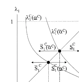
We now examine the effects of the lawyer’s costs on the PBE. Specifically, we compare the results whenalllawyers havec50 with those whenalllawyers havec5C.0: for simplicity, the two situations are assumed not to coexist. The lawyers’ “type” is common knowledge.16Using obvious notation to distinguish settlement offers, mixing probabil-ities and values oflwhenc50 and whenc5C, we have
15We can easily solve forpˆ . Defineg [(h1c/a)[(11 d)(x#2x)1(h1c/a)]. Thenpˆ5 g[d(x#2x)21 g]21[
(0, 1).
16As noted in the Introduction, we can interpret the situation whenc5Cas involving a conflict of interest between
plaintiff and lawyer. Whenc50, the lawyer faces exactly the same bargaining incentives as her client would if he were conducting the litigation. Accordingly, no conflict is present and the lawyer receives and accepts exactly the same settlement offers as the plaintiff would. Whenc5C, however, the lawyer faces costs of bargaining that her client would not. It is now possible that her negotiating position will differ from that which her (non-cost-bearing) client would choose.
PROPOSITION2: Holdingaconstant,St0.St,C; S#t0.S#tC; a0 .aC;ltC. lt0; t51, 2.
PROOF: This follows directly from setting c 5 0 and c 5 C . 0 in (1)–(5) and comparing the outcomes.■
To understand this result, begin withSt. Whenc50, there are no marginal costs of
continuing to bargain. In one sense, this strengthens the plaintiff’s lawyer’s bargaining position and, for any given damage level, forces a higher settlement offer from the defendant [see (1) and (2)]. In turn, this lowers l2 [i.e., l2C . l20] because the defendant has no costs to extract in his settlement offer, so his relative cost of a low-damage offer in Period 2 falls. The value ofashows how a lawyer representing a low-damage plaintiff reacts to this. Because her intention is to induce a settlement offer based on x#, bearing no costs means that she must “work hard” to convince the defendant that he faces a high-damage plaintiff in Period 2. She does this by accepting an offer that a high-damage plaintiff’s lawyer would certainly reject (i.e.,S1) with higher probability because this makes the rejections she plays more credible signals that she indeed represents a high-damage plaintiff: hence, a0 . aC. Finally, the tendency for
“zero cost” lawyers to accept low-damage first period offers more frequently increases the set of parameters for which such offers are forthcoming: hence,l1C. l10.
Thus, bearing costs has two effects on a contingent fee lawyer’s behavior. First, she accepts lower offers given the level of damages (thecost effect). However, second,when representing a low-damage plaintiffshe is able to bargain hard because costly actions convey more credible signals than costless ones. Because the cost-bearing lawyer risks more by rejecting an offer, the rejection is a more credible signal that she represents a high-damage plaintiff, even though she does not (thehard bargaining effect).
Having established that cost-bearing and contingent fees can produce this effect in a dynamic setting, we now wish to see how this influences the timing and size of settle-ment. Before moving on we can, as before, definepˆ0andpˆCas the critical values ofp
that determine whether the defendant offersS1orS#1at the start of bargaining. It follows from Proposition 2 thatpˆC. pˆ0.17
III. Price Competition Among Lawyers
Propositions 1 and 2 give us the information required to compute the probability of settlement and the plaintiff’s payoffs, depending on his lawyer’s costs. However, we must first ensure that the value ofais consistent across the two types of lawyer. One way to do this is to assume that, before they discover the plaintiff’s damage level, lawyers compete for the case on the basis of price, with each bidding a value ofaat which they will take the case.18If each has a reservation utility of
V, then price competition will continue until the value ofa equates lawyers’ex ante payoffs from the case with the reservation level. We proceed in this way, calculating the endogenous values ofa.
If lawyers are sufficiently well informed, they can solve for the equilibrium of the case, depending on the type of plaintiff they represent, by backwards induction. They will,
17In fact, proving the existence of thesepvalues is made more complicated by the endogenous values ofa
computed in the next section. We can solve forpˆ0directly by substitutingc50 intopˆ in n. 15. However, whenc5
C,acan become a function ofpand the value(s) ofpˆCbecome the real root(s) of a cubic, which are hard to solve
for analytically. We can still confirm the existence of a uniquepˆC, but we leave the rather mechanical analysis for the
Appendix.
18Both Danzon (1983) and Swanson (1991) note that a particular advantage of contingent fees, over input-based
therefore, know whether a high- or a low-damage offer can be expected in Period 1, conditional on the type of plaintiff they represent. Given this, there will be competitive values ofaforc[{0,C}, and based on whether the lawyer expects a high-damage offer or a low-damage offer in Period 1.19Using the superscript “c” to emphasize that values vary withc[{0,C}, we call thesea#candac, respectively. It is straightforward to confirm
(see the Appendix) that these are given by
a#c5V1~11d1d
Notice that these PBE fees compare the costs of taking the case, from the lawyer’s perspective, with the benefits in terms of the (expected) damages to be shared between lawyer and client. Ranking the values ofa(again using obvious notation), we have
aC
.a0va#C
.a#0. (6)
As we would expect, the plaintiff’s lawyer needs a higher percentage fee to cover her opportunity costs (1) the lower is the settlement offer she anticipates, and (2) the longer she expects to have to continue bargaining (i.e., when she expectsS1crather than S#1c).
IV. Settlement Timing and the Plaintiff’s Payoffs
We now compare settlement timing and the plaintiff’s payoffs underc [{0, C}. The plaintiff’s payoffUPis a function ofc,S
1anda1. Using an overbar (underbar) to signify whether the plaintiff is high- (low-) damage, and the subscript “c” as before, we have
U#P(c,S
From (8), the high-damage plaintiff always receives a payoff based on x#: he either receives a high-damage settlement offer (when p , pˆc) or his lawyer refuses all
low-damage ones and waits for a high-damage trial award (whenp . pˆc). As a result,
he may only benefit indirectly from hard bargaining, through its effect ona. In contrast, the low-damage plaintiff either receives a high-damage offer immediately (p , pˆc) or
her lawyer “haggles” in response to a low-damage one (p . pˆc).
Combining Propositions 1 and 2 with (6), (7) and (8) yields the results in Table 1. This distinguishes three regions for the initial value ofp. Whenp[(0,pˆ0)ø(pˆC, 1), both types of plaintiff receive higher payoffs whenc50. There are two reasons for this. First, in both regions, thecost effectoperates but there is nohard bargaining effectto offset it (potentially) for low-damage plaintiffs. In particular, whenp , pˆ0 the first offer is based onx#, whetherc50 orCwhile, whenp . pˆC, the first offer is based onxwhether
c 5 0 or C. However, whenc 5 C, the defendant’s settlement offer is lower by the
19Interestingly, if the lawyer’s “cost-type” were not known by the defendant, the competitive fee level could signal
amount of the lawyers’ future costs, which can be extracted through the offer [see (1) and (2)]. Thus, holding damages fixed, offers are lower underc 5C. This creates a second effect: because offers are lower when c 5 C, the competitive contingent fee percentages are higher [see (6)], meaning that both types of plaintiff pay a larger fraction of the (smaller) sum recovered.
Interestingly, in this joint region, there is no prospect of positive bargaining costs increasing the speed of settlement: settlement is either instant for certain (whenp , pˆ0), or instant with a higher probability underc50 (whenp . pˆC) (see Figure 3). In
the former case, this is because an offer based onx#is received in all cases. In the latter, it is because the cost-bearing lawyer’s hard bargaining fails, but involves acceptingS1C with a lower probability. Thus, contrary to policy debate, whenp[(0,pˆ0)ø(pˆC, 1), a conflict of interest caused by bargaining costs under contingent fees can emerge, but not as a result of the lawyer achieving speedy settlement.
Now consider intermediate values ofp, i.e., p[ (pˆ0, pˆC). Here, the cost-bearing lawyer’s hard bargaining succeeds in inducing a high-damage settlement offer from the defendant, while the lawyer bearing no costs induces a low-damage offer. Thus, it is now
TABLE1. The effects of the plaintiff’s lawyer’s costs
Value ofp p , pˆ0 p
ˆ0, p , pˆC p . p
ˆC
Plaintiff’s preference
H
x5x x5x#c50 c[{0,C} c50
c50 c[{0,C} c50
Pr (settle in Period 1) when
H
c50 c 5 C1 pa0 pa0
1 1 paC
possible for a low-damage plaintiff to gain from hard bargaining: this happens when the higher level of damages received compensates the reductions in settlement demands due to the extraction of legal costs (i.e., the hard bargaining effect dominates the cost effect). Both types of plaintiff can also benefit to the extent that the high-damage offer allows the lawyer to bid a lower contingent fee percentage underc5C: as (6) shows,
a#Cva0. Finally, there is a higher probability of speedy settlement as a result of the conflict of interest because high-damage offers are accepted for certain.
Discussion
These results indicate the presence of opposing factors when considering whether a self-interested lawyer will settle a contingent-fee case sooner when facing litigation costs than when these are not present, and whether her client suffers in such circumstances. The ambiguity in settlement timing is because bargaining harder involves rejecting more low-damage offers as well as inducing more (acceptable) high-damage ones. Whether the plaintiff is better off when his lawyer faces costs will vary from case to case, although it is worth noting that only a low-damage plaintiff can benefit from the direct effects of hard bargaining. The principal influences on this preference are the relative magnitudes of the cost and hard bargaining effects, which work in opposite directions on the size of the settlement offers, and the degree of uncertainty surrounding whether the plaintiff is high or low damage (i.e., the value ofp). The cost and hard bargaining effects tend to have reinforcing effects through their influence on the contingent-fee percentage.
Notice that, as the plaintiff’s preferences fluctuate, so too does the situation that maximizes theex antejoint welfare of the plaintiff and his lawyer (given by the sum of their payoffs). This is because, with the lawyer held to reservation utility, this joint payoff varies directly with the plaintiff’s. Of course, whenp¸(pˆ0,pˆC), this joint welfare is
harmed by the presence of bargaining costs and contingent fees.
Influence of Case Characteristics
Finally, we analyze how the characteristics of the case in question (p,C,h,x#,x,V) affect the likely success of hard bargaining.20Two issues are considered: when is hard bar-gaining more likely to induce a high-damage initial offer? (i.e., when doespˆCincrease?)
and when is this more likely to benefit the plaintiff?21
The circumstances in which hard bargaining is likely to succeed can be read from the bottom line of Table 2 (derivations are in the Appendix); only a mean preserving
20We assume that a change in parameter values does not shift the negotiation from the Pareto optimal equilibrium,
that witha15a.
21By “more likely” we mean that a larger set of parameters is consistent with the event. TABLE2. Influences onpˆCandpˆ0
Variable: C h V
Increased mean damages (spread fixed)
Increased damage spread (mean fixed)
pˆ0 0 1 0 0 ?
pˆC 1 1 2 1
spread of damages has an ambiguous effect onpˆC. Elsewhere, higher costs for either
side (Candh), a higher arithmetic mean of damages (holding spread constant), and a lower opportunity cost for the plaintiff’s lawyer all increase the set of parameters conducive to a high-damage offer under hard bargaining. The role played byChere has already been explained. Higher average damages make the defendant keener to offer
S#1Cbecause they lowera#Cand allow more future costs to be extracted in the settlement offer [see (1) and (2)]. This is also the reason why an increase in the lawyer’s oppor-tunity cost on the case weakens her hard bargaining position. Finally, it is not surprising that a defendant facing higher costs is keen to settle in Period 1. As Table 2 shows, the first three of these effects are due to hard bargaining (they do not occur whenc50); the fourth occurs regardless of the lawyer’s bargaining stance.22
It is difficult, without an explicit expression forpˆC, to derive unambiguous
compar-ative static results for the effects of case characteristics on the plaintiff’s payoffs. However, Table 1 shows that a necessary condition for either plaintiff to benefit from hard bargaining is p [ (pˆ0, pˆC). Therefore, changes that widen this region are necessary—not sufficient—to make hard bargaining more likely to benefit plaintiffs. Table 2 shows that this is unambiguously the case for three of the factors that make hard bargaining more likely to succeed: higherC and average damages and lowerV. How-ever, as we have seen, raising the defendant’s costs weakens him, regardless of the lawyer’s strategy and, therefore, has an ambiguous effect on the necessary condition for plaintiffs to benefit from hard bargaining.
V. Conclusions
One reason, given by some policy makers and supported by previous literature, for concern over the effects of contingent fees for lawyers is that they provide incentives for lawyers to settle cases earlier, and for less, than clients would wish. In particular, this concern has focused on the lawyer’s desire to prevent accumulated bargaining costs from consuming her share of the available damages. This paper has shown that such a view is too simplistic: in a dynamic setting, bargaining costs produce strategic influences that work in opposite directions, thereby complicating the role of costs and contingent fees.
Certainly, holding the level of damages constant, a cost-bearing contingent fee lawyer’s self-interest will lead her to receive and accept lower settlement amounts than her client would wish [thecost effectidentified byinter aliaMiller (1987)]. In a compet-itive market for lawyers, this may further damage the plaintiff by increasing the con-tingent fee percentage required by the lawyer to cover opportunity costs on the case. However, when lawyers have private information and the opportunity to influence future periods of bargaining, these bargaining costs can play a strategic role. Thus, when the lawyer bears costs, her rejections of a settlement offer are more credible signals that she represents a severely damaged client than when she bears no costs (the
hard bargaining effect). Accordingly, bearing costs allows the lawyer to bargain harder and may induce a higher settlement offer. Which of these two factors dominates has been shown to depend on the characteristics of the case: the size of the lawyer’s costs themselves, the spread and level of damages involved, their initial probability of occur-ring, and level of the defendant’s costs. The central policy lesson, however, is that
22Technically, the difference is due to whether or notc/aappears inl 2
c, which it does not whenc50. Conversely,
contingent fees need not be dismissed for giving lawyers self-interested incentives: in some circumstances, this may be exactly what their clients need.
There are many ways in which the paper could be extended to improve our knowl-edge of how contingent fees affect litigation behavior. The model ignores several features that are relevant to the question at hand. For instance, plaintiffs are often risk averse, and lawyers can often influence court decisions. Because there is reason to believe that contingent fees have risk sharing and signaling properties, it would be appropriate to incorporate risk and court error into the model; by allowing lawyers to signal to the court, this may enhance the effects of hard bargaining under costs and contingent fees. In turn, this would make a consideration of the effects of contingent fees under other cost allocation rules—like the English one—more interesting. A further issue concerns the comparative effect of contingent fees on litigation relative to other fee contracts: even if contingent fees operate imperfectly, do they dominate other arrangements?
It would also be interesting to study the optimal contract between lawyer and client in a dynamic pretrial bargaining environment. This raises the interesting issue of renegotiation of the fee contract upon receipt of a settlement offer. For example, if the defendant’s side has private information, there may be offers that become acceptable to the plaintiff and his lawyer (as this information emerges), but that the lawyer would reject under the original contract.
Finally, we might consider the role of contingent fees in richer dynamic bargaining contexts, particularly ones with endogenous delay and two-sided information asymme-tries. Although our model indicates that the results here are likely to be complicated, it also suggests that the strategic incentives within a given bargaining environment are important to understanding how fee arrangements affect settlement timing and settle-ment amounts.
Appendix: Contingent Fees and Litigation Settlement Proof of Proposition 1
LetS˜1be the minimum Period 1 offer that a low-damage plaintiff’s lawyer would accept whenS25S#2. Therefore,S˜1satisfies
aS˜12c5ad2
S
x#2 ca
D
2c2dcso that S˜1 5 S#1. Also, define D [ x# 2 x. Finally, define the defendant’s payoff as a function of the Period 1 settlement offer and the low-damage plaintiff’s lawyer’s re-sponseUD(S
1,a1). Therefore,
UD~S#
1, 1!52~S#11h!
UD~S
1,a!52~paS11~12pa!S#2!2h2d~12pa!h.
The proof proceeds by examining the parties’ strategies in two situations:p , l2and p . l2.
m; p~12a! p~12a!112p.
Because his high-damage opponent playsa#1 50@S,S#1, we must havem#p. Thus
(by definition ofl2), ifp , l2, the defendant will offerS#2in Period 2. Anticipating this, the low-damage plaintiff’s lawyer will not acceptS1,S˜1, so the defendant must offerS#1, which both types of plaintiff accept. This yields the defendant the payoffUD(S#1, 1).
(2)p . l2: Again, the defendant can offerS#1and settle the case. ConsiderS1[[S1, S#1), which means that the high-damage plaintiff’s lawyer playsa#150. The low-damage plaintiff’s lawyer cannot playa1. a, as this would induce m , l2 andS#2, which she would certainly prefer. Suppose she plays a1 ,a, which inducesm . l2, so thatS2 is offered. Accordingly, ifS1 [(S1,S#1) she would playa151, a contradiction. ForS15 S1, anya1[[0,a] will suffice. As explained in the text, we focus on Rasmusen’s Pareto optimal focal pointa1 5a. If mixing, she must be indifferent between accepting and rejecting S1. This must mean that her opponent is also mixing between S2 andS#2. Lettingqdenote the defendant’s probability of playingS#2, we have
aS12c5qaS#21~12q!adS22c2dc
fq5
S12dS21d c a
d~S#22S2! .
To determineS1andS2, we note that the defendant’s expected payoff fromS1[[S1, S#1) is given by2[paS1 1(12 pa)dS2] 2h2 (12 pa)dh, using the fact that he is indifferent in the second period betweenS2andS#2. This is clearly minimized byS1, so that (from the equation forq) he playsS2 in Period 2.
Thus, the Pareto optimal PBE depends on the parameter values. The defendant can offerS#1and the plaintiff’s lawyer playa15a#151, generating the defendant an expected payoff of UD(S#
1, 1). Alternatively, the defendant can offer S1 and the plaintiff’s lawyer playa15a,a251;a#15a#250, giving the defendant an expected payoff of UD(S1, a). The equilibrium outcome will depend on which yields the defendant the highest expected payoff. Settlement will definitely occur in Period 1 if UD(S#
1, 1) . UD(S1,a). Substituting in for the relevant settlement amounts and rearranging tells us that this implies
~12pa!
S
h1ca
D
.padDf
h1 c
a
a
S
dD1h1ca
D
;l1.p.
PBE Fee Percentages (from Section III)
Consider first the values ofawhen the lawyer expects to face a high-damage settlement offer. Her expected payoff is the same regardless of whether she expects to represent a high-damage or a low-damage plaintiff. Denoting the payoff from these asU#L(c,S#
1
Now suppose the lawyer expects to receive a low-damage settlement offer in Period 1. Here, her expected payoff depends on whether she expects to represent a high-damage or a low-damage plaintiff. When representing a high-damage plaintiff, the offer is rejected, the case goes to trial, and the lawyer receives
U#L~c,S1c!5acd2x#2c2dc2d2c.
When she represents a low-damage plaintiff, either the first or second period offer is accepted. The lawyer’s expected payoff is
UL~c,S
In Proposition 1, we were able to calculate a unique value of p(i.e.,pˆ ) at which the defendant switched between offering S1 andS#1. This was easily done because awas assumed to be exogenous. Now thatahas been made endogenous, we need to check whether such a unique value ofpremains underc[{0,C}. The problem is that, with two pairs of equilibrium values fora— depending onc, i.e., {a0,a#0} and {aC,a#C}—there
are two pairs of l1 functions: with obvious notation {l10(a0), l01(a#0)} and {l1C(aC), l1C(a#C)}. Given thatpˆ is the root ofl1(p)5 p, the multiplel1functions might imply multiple “switching probabilities.” In fact, we can show that this is not the case.
To begin, the case ofpˆ0is straightforward. With
c50,adoes not enter intol1, and we have
l10~a0!5l10~a#0!5 h a0~dD1h!.
It is easy to check that this has a unique root, with the value implied by n. 15 in the text. To establish the existence and uniqueness ofpˆCwe first note that the endogenous
l1C~a#C!5
h1 C
a#C
aC~a#C!
S
D1h1 C
a#C
D
and l1C~aC!5
h1 C
aC
aC~aC!
S
D1h1 C
aC
D
where we have recognized the dependence ofa1Conaas well. We now do two things: first, we examine the boundaries within which pˆC must lie; then, we establish the
existence and uniqueness of pˆC within these. These are done, respectively, in the
following two lemmas.
LEMMA1: (1)l1C(a#C)andl1C(aC)both slope down inpand have unique fixed points.(2) l1C(a#C). l
1 C(aC).
PROOF: (1) It is easy to confirm that]l1C(aC)/]p ,0. (2) This is easily checked by rearrangement.■
We shall refer to the fixed point ofl1C(aC) aspˆ
1
C, and to that ofl
1
C(a#C) aspˆ
2
C. Clearly,
pˆ2C. pˆ1C, as depicted in Figure A1.
Figure A1 tells us that, whenp , pˆ2C, the defendant will offer S#1C based on a#C, S#1C(a#C), and whenp . pˆ1C, the defendant will offerS1Cbased onaC,S1C(aC).1However,
23Whenp , pˆ 1
C, the defendant will make a high-damage offer regardless of the value ofa. As a result, the value
this leaves us unclear as to what the defendant will do whenp[(pˆ1C,pˆ2C). As depicted in Figure A1, in this region, the defendant would like to offer S#1C(a#C) and S1C(aC). Which will be offered will be decided by which yields the defendant the highest payoff. We wish to show that there is at most one value ofp, at which the defendant switches between these offers on the interval (pˆ1C,pˆ2C). Lemma 2 states a result here.
difference between the defendant’s payoffs from the two competing offers in (pˆ1C,pˆ2C). We wish to show thatc(p) has a unique root on (0, 1).2
We shall focus on this expression.
Notice first thatc(0) 5 2dh 2 dC/aC ,0, because aC5 a#Cwhen p 50. Next,
considerc(1)5 d2D 1(11 d)dC[1/a#C21/aC] .0 sinceaC. a#Cwhenp 51.
Therefore,c(p) increases on [0, 1]. If we can show that this happens monotically, we will have established thatc(p) has a unique root on this interval.
Differentiating Equation (A1) with respect topyields
]c~p!
suppressed the functional notation on aCfor convenience. Because aC 5 1 2 (1 2
p)(h1C/aC)/pD, we have
ofawill bea#Cand the settlement offer will build this into the analysis. Similar reasoning confirms the offers made
whenp . pˆ2C.
Substituting this into Equation (A2) and rearranging gives
The first term here is positive, as is daCu; the bracket is harder to sign. Define this
bracket as
dCaCD
Lemmas 1 and 2 have established the existence of a unique value ofpat which the defendant will switch from offeringS1C(aC) to offeringS#1C(a#C): this ispˆCfrom Section we have seen and its derivatives are easily determined). Thus, we focus onc(p), from Equation (A1), to which we apply the implicit function theorem (IFT). It is useful to begin by recalling the expressions foraC,a#Cand
The Effects of Plaintiff Costs(C)
Using this, and Equation A1, we have
]c
M),0. The remaining terms are also negative (in total) from Equation (A3) and the fact thatpaC,1. Therefore,
]c ]C,0f
dpˆC
dC .0.
The Effects of Defendant Costs(h) Given Lemma 2, this is determined by]c/]h. From Equation A1:
]c
The Effects of Lawyer Opportunity Costs(V) We are interested in]c/]V. Start by noting
Therefore, using this and Equation (A1)
plus Equation (A4) and the fact thatpaC,1, we have
]c
]V.0f dpˆC
dV ,0.
The Effects of Higher Mean and Spread of Damages
The mean level of damages is given by
xm
5x #1x
2 .
To model an increase in the mean, with no change in spread, and a mean-preserving increase in spread, we must, therefore, recognize that x# and x will need to move simultaneously. For example, we can consider the effects of dx#, bearing in mind the subsequent effects of dx/dx#. In particular, for an increase in mean (no change in spread), we havedx/dx#51, and for a mean-preserving increase in spread we havedx
/dx# 5 21.
Bearing this in mind, we begin by noticing that, in general,
]
S
CTherefore,
dxˆC
dxm
U
Dfixed .0.We examine a mean-preserving increase in spread by substituting Equations (A5) and (A6) into (A7), and settingdx/dx#5 21. It is easy to confirm that the resulting version of Equation (A7) cannot be signed, implying thatdxˆC/dDu
xmfixedv0.
References
BARCOUNCIL. (1989).The Quality of Justice: The Bar’s Response. London: General Council of the Bar. BENSON, LORDH. (1979). London:Royal Commission on Legal Services: Final Report; Cmnd 7684 HMSO. CRAMTON, P. (1984). “Bargaining with Incomplete Information: An Infinite-Horizon Model with
Con-tinuous Uncertainty.”Review of Economic Studies51:579 –593.
DANA, J.,ANDK. SPIER. (1993). “Expertise and Contingent Fees: The Role of Asymmetric Information in Attorney Compensation.”Journal of Law, Economics and Organisation9:349 –367.
DANZON, P. (1983). “Contingent Fees for Personal Injury Litigation.”Bell Journal of Economics14:213–224. DAUGHETY, A.,ANDJ. REINGANUM. (1994). “Settlement Negotiations with Two-Sided Asymmetric Infor-mation: Model Duality, Information Distribution and Efficiency.”International Review of Law and Economics14:283–298.
DIXIT, A. (1980). “The Role of Investment in Entry-Deterrence.”Economic Journal90:95–106.
DONOHUE, J. (1990). “The Effects of Fee-Shifting on the Settlement Rate: Theoretical Observations on Coase, Costs, Conflict and Contingency Fees.” Working Paper No. 127, Centre for Studies in Law, Economics and Public Policy, Yale Law School, New Haven, CT.
EMONS, W. (1998). “Expertise, Contingent Fees and Insufficient Attorney Effort.” Paper presented at the 15th Annual Conference of the European Association of Law and Economics, University of Utrecht, September 24 –26.
FUDENBERG, D.,ANDJ. TIROLE. (1983). “Sequential Bargaining with Incomplete Information.”Review of Economic Studies50:221–247.
FUDENBERG, D.,ANDJ. TIROLE. (1991).Game Theory.Massachusetts: MIT Press.
GENN, H. (1981).Hard Bargaining: Out of Court Settlement in Personal Injury Actions. Oxford: OUP. GRAVELLE, W.,ANDM. WATERSON. (1993). “No Win, No Fee: Some Economics of Contingent Legal Fees.”
Economic Journal103:1205–1220.
HALPERN, P.,ANDS. TURNBULL. (1983). “Legal Fee Contracts and Alternative Cost Rules: An Economic Analysis.”International Review of Law and Economics3:3–26.
HARRIS, D., M. MACLEAN, H. GENN, S. LLOYD-BOSTOCK, P. FENN, P. CORFIELD,AND Y. BRITTAN. (1984). Compensation and Support for Illness and Injury. Oxford: OUP.
HAY, B. (1995). “Contingent Fees and Settlement.” Discussion Paper No. 161, Programme in Law and Economics, Harvard Law School, Cambridge, MA.
KAKALIK, J., M. SELVIN,ANDN. PACE. (1990).Averting Gridlock: Strategies for Reducing Civil Delay in the Los Angeles Superior Court, R-3762-ICJ. Santa Monica, CA: Institute for Civil Justice, RAND.
KRITZER, H. (1990).The Justice Broker: Lawyers and Ordinary Litigation. Oxford: OUP.
KRITZER, H., A. SARAT, D. TRUBEK, K. BUMILLER,ANDE. MCNICHOL. (1984). “Understanding the Costs of Litigation: The Case of the Hourly Fee Lawyer.”American Bar Foundation Research Journal559 – 604. Law Society. (1989).Striking the Balance: the Final Response of the Council of the Law Society on the Green Papers.
London: Council of the Law Society.
Lord Chancellor’s Department. (1989).Contingency Fees, Cm 571. London: HMSO.
MACKINNON, F. (1964).Contingent Fees for Legal Services. Chicago: Aldine Publishing Company. MILLER, G. (1987). “Some Agency Problems in Settlement.”Journal of Legal Studies16:189 –215. RASMUSEN, E. (1989).Games and Information: An Introduction to Game Theory.Oxford: Basil Blackwell. RICKMAN, N. (1994). “The Economics of Contingent Fees in Personal Injury Litigation.”Oxford Review of
RUBINFELD, D.,AND D. SAPPINGTON. (1987). “Efficient Awards and Standards of Proof in Judicial Pro-ceedings.”RAND Journal of Economics18:308 –315.
RUBINFELD, D.,ANDS. STOTCHMER. (1993). “Contingent Fees for Attorneys: An Economic Analysis.”RAND Journal of Economics24:343–356.
SCHWARTZ, M.,AND D. MITCHELL. (1970). “An Economic Analysis of the Contingent Fee in Personal Injury Litigation.”Stanford Law Review22:1125–1162.
SHAVELL, S. (1982). “Suit, Settlement and Trial: A Theoretical Analysis Under Alternative Methods for the Allocation of Legal Costs.”Journal of Legal Studies11:55– 81.
SMITH, B. (1992). “Three Attorney Fee-Shifting Rules and Contingency Fees: Their Impact on Settlement Incentives.”Michigan Law Review90:2154 –2187.
SPIER, K. (1992). “The Dynamics of Pretrial Negotiation.”Review of Economic Studies59:93–108. SWANSON, T. (1991). “The Importance of Contingency Fee Arrangements.”Oxford Journal of Legal Studies
11:193–226.