Enforcement System
FRANK VANTULDER ANDABRAHAM VAN DERTORRE Social and Cultural Planning Office, Rijswijk, The Netherlands
E-mail address: [email protected]
I. Introduction
In the Netherlands, as in many other countries, crime is an important social and economic issue. What are the causes of crime trends in the Netherlands? And how can crime be countered by the law enforcement system in the most effective and efficient way? What will be the inmate population of the prison system in the years to come?1 These are key questions for policymakers. Economists of crime try to answer these questions, continuing a tradition that goes back to Becker (1968).
The Social and Cultural Planning Office has developed a model of those parts of the Dutch law enforcement system that are relevant to the above questions. This article describes that model, which uses macroeconometric estimations to link the crime rates, the responses of the law enforcement system, and the inputs into that system. These estimations are then used to formulate forecasts and scenarios for the Dutch law enforcement system for the period 1996 to 2002. Questions that the model can answer are: Is the law enforcement system able to produce more repression with the same funding? What additional resources does the government need to apply to reduce crime by 1%, given an efficient production of repression and given specific demographic and social developments?
II. A Macroeconomic Model for Crime and the Law Enforcement System
Figure 1 sketches the principal flows within the law enforcement system. Crime depends on factors such as the functioning of the police, the public prosecutions department, the administration of justice, and the prison system. These institutions, respectively, clear up crimes, prosecute and judge criminal cases, and lock up criminals. Their outputs may affect the behavior of potential criminals. Potential criminals can be influenced by the likelihood of being arrested, the likelihood of being punished, and the severity of the punishments dealt out (i.e., the amounts of fines and the lengths of prison sentences).
1The Ministry of Justice uses the model presented here in the process of planning the capacity of the prison system. The development of the model is still going on. We are presenting here a preliminary version.
International Review of Law and Economics 19:471– 486, 1999
In formulating a macroeconomic model for a law enforcement system, one must bear in mind that action in one part of the system has consequences for other parts. If the police clear up more crimes, if the public prosecutor receives more cases, and if the cases are not dropped, the judge gets more cases too. Subsequently, if more prison sentences are meted out, more cells are needed. The greater probability of being
arrested by the police and the fact that more criminals are in prison (incapacitation effect) will probably reduce crime. This in turn will affect the activities of the police. From this point the reasoning can be repeated. We therefore ultimately need a simul-taneous and interrelated model.
The full model incorporates the following relationships:
1. Relationships of the number of victimizing crimes of various typesper capitato: • the probability of being arrested
• the probability of being punished if arrested
• the probability of being locked up in prison if punished
• the average term of imprisonment if applied (as well a deterrence as an incapac-itation effect)
• demographic and socioeconomic variables
2. Relationships modeling the production structure of the police force. The endoge-nous output variables are the numbers of crime solutions of all the types of crimes considered (victimizing and victimless). Inputs are fixed by the government and are, thus, treated here as exogenous to the system.
3. Relationships modeling the production structure of the public prosecutions depart-ment and the judicial system. In the Netherlands these institutions form one organization. This organization “produces” guilty verdicts. As with the police, inputs are fixed by the government and are, therefore, treated as exogenous to the system. 4. Functions that describe the behavior of public prosecutors and judges in terms of the percentages of prison sentences of various time lengths for various types of crime.
Relationships 1 to 4 will be estimated empirically by time-series analyses. The data have been collected mainly from statistical publications of the Dutch Central Office for Statistics.
The rest of this article discusses the above relationships and their estimations. Finally, some simulations are presented.
III. Analyses of Crime
This section presents a time-series macroeconomic model of crime. The selection of explanatory variables is based both on criminological and economic theoretical notions regarding the causes of crime. Of course, we restrict ourselves to those notions that are relevant and can be “translated” into variables at a macroeconomic level.
The criminological theoretical notions can be roughly divided into three types. The first type stresses the importance ofnormsor the absence of them. Social instability and cultural shocks may play a role here. Variables representing this type of theoretical notion are: age (proportion of young men); family status (proportion of divorced people); cultural background (proportion of non-native people); and number of drug addicts.
The second theoretical approach accentuates the relevance of social position and legal opportunities for the potential offender. Variables coming into play here are: unemployment (proportion of unemployed) and (legal) income (average real net income).
(approximated by the Theil measure of income inequality) and to the presence of cars (number of motor vehiclesper capita).
The economic approach stresses the importance of legal opportunities to crime and the possibilities of making lucrative gains in the illegal circuit. These are influenced both by the opportunities provided by potential victims and the (expected) reaction of the law enforcement system, resulting in the crime clear-up rate and the probability and severity of punishment.
It is clear that there is not always a unique relationship between explanatory variables and theoretical notions. Legal opportunities play a role both in the second crimino-logical and in the economic approaches. So, the results are not meant to test one theoretical notion against another. Rather, it is our intention to link crime trends at the macro level as well as possible to trends in society of a demographic, social, and economic nature that are autonomous from the law enforcement system on the one side and from the reaction of the law enforcement system on the other side. Note also that average income as income inequality are explanatory variables in the analysis.
The effects of the probability of arrest (expressed below in terms of crime clear-up rates), the probability of punishment, the probability of imprisonment, and the length of the probable prison sentence express themselves in two different ways. They may have a preventive ordeterrent effect, because a greater probability of being caught or the prospect of a higher sentence may cause potential offenders to decide not to commit a crime. There may also be anincapacitation effect, because imprisonment prevents offend-ers from reoffending for the duration of their term in prison.
In the empirical literature, the distinction between these effects has not always been drawn successfully. See Wolpin (1978)2and Van Tulder (1994) for exceptions. We will not explicitly distinguish and estimate these two types of effects in the time-series model we use here. The probability of receiving a prison sentence and the expected term of the sentence incorporate both effects. In a cross-sectional analysis by Van Tulder (1994), in which the two effects were separately treated, 100% of the total effect seemed to consist of the incapacitation effect (so that the deterrent effect was zero).
Crimes can be broken down into two categories: those that victimize and those that do not. Violence and theft immediately produce victims. Drunk driving and crimes against drug laws generally do not.3 In the case of the so-called victimizing crimes, registration by the police depends to a great extent on the informing behavior of the victims, and not all registered crimes are cleared up. In contrast to victimizing crimes, the number of registered victimless crimes is almost exactly equal to the number of crimes cleared up by the police. So the clear-up rate is nearly 100%. However, the real level of the victimless crimes remains unknown, because there are no victims to inform the police and because the police do not observe all the crimes themselves. For this reason, we have restricted our macro time-series analyses to four types of victimizing crimes. We have distinguished violence (including serious sexual crimes), petty thefts, aggravated thefts, and “other crimes” (with drunk driving and crimes against drug laws excluded).
To avoid multicollinearity and cointegration problems, each relationship is estimated
2Some tried to estimate the incapacitation effect by theoretical probability models, e.g., Shinnar and Shinnar (1975). Cohen (1978) presents an overview.
in first differences.4 In addition, to avoid “simultaneity bias,” the relationship is esti-mated with a two-stage least squares technique, namely, the instrumental variables technique.5Table 1 shows the results of our time-series analyses. Because the model has been estimated in logarithms, the coefficients are elasticities.
Several specifications were tried for the above relationships. In these analyses the constant term never became significant, and because a constant term representing a trend has no theoretical justification, it has been omitted. In addition, no variables with unexpected signs were significantly correlated. All variables the coefficients of which had incorrect signs have been omitted from the estimations presented above, so that only those with the right sign remain.
For violence, petty (simple) theft and other crimes, the coefficient of the clear-up fraction was significantly negative. This means that a rise in the clear-up rate for one of
4For violence we succeeded in constructing a long-term relationship in levels and first differences which meets the cointegration criteria. For the other types of crime we have not yet managed to construct such a relationship. We have therefore had to restrict ourselves to first differences.
5The instruments used are all independent variables of the whole model.
TABLE1. Analysis of recorded crimeper capita, 1957–1995
Violence Petty Thefts Aggravated Thefts Other Crimes
Clear-up rate 21.65 (2.7)* 20.64 (2.3)* — 20.64 (2.5)*
Probability of being punished 20.59 (1.1) — — —
Probability of being imprisoned
Divorcedper capita 0.32 (1.2) 0.13 (0.7) 0.11 (0.3) 0.34 (2.0)*
Non-nativesper capita — — 0.35 (0.8) —
Unemployedper capita‡ 0.26 (1.6) 0.11 (0.6) 0.60 (2.2)* 0.11 (0.9) Average incomeper capita 0.04 (0.2) 20.09 (0.2) 20.67 (0.9) 20.21 (0.6) Theil coefficient 0.98 (2.2)* 0.16 (0.4) 0.51 (0.9) 0.38 (1.5) Clinic admissions of drug addicts
per capita
— 0.21 (2.8)* 0.24 (2.0)* —
Motor vehiclesper capita — 0.28 (1.1) 1.10 (2.4)* 0.14 (0.7)
Number of observations 39 39 39 39
R2 0.467 0.597 0.465 0.616
R2(adjusted) 0.347 0.506 0.322 0.514
Durbin-Watson 2.11 1.71 1.96 2.16
Test for stability (F-test)§ 1.39 1.53 0.49 1.65
Dickey-Fuller test\ 2
6.29* 25.74* 26.3* 26.46*
Notes: See Appendix for the mathematical specification of the whole model. A simultaneous estimation procedure is used. The method of estimation is “2-stage least squares,” namely, the instrumental variables technique. Coefficients marked with * are significant at 5% level,tvalues in brackets.
†As well a deterrence as an incapacitation effect. ‡Including the number of incapacitated. §F
0.9552.37 for all types of crime. This test assesses stability by dividing the set into two parts and estimating both parts separately.
those types of crime would reduce the level of that type of crime. An increase in the clear-up rate by 1% would lead to a crime decrease of 1.65% for violence, 0.64% for simple theft, and likewise 0.64% for other crimes. The probability of being punished and the probability of being imprisoned never achieve significant coefficients. The average term of imprisonment is significant only for violence (0.30).
The results are in agreement with the literature, which finds generally significant elasticities of the probability of arrest or sanctions on crime and somewhat lower elasticities of severity of punishment [see Eide (forthcoming)].
With respect to the demographic and socioeconomic variables, the following obser-vations can be made: Rising income inequalities (Theil coefficient) have a stimulating effect on violence. A growth of 1% of the Theil coefficient leads to a growth of 0.98% in violence. The pattern in petty thefts is significantly affected by changes in the number of young men and the number of drug addicts (roughly approximated by the numbers of clinic admissions). A rise in the numbers of young men or drug addicts by 1% boosts the number of simple thefts by 2.35% and 0.21%, respectively. An interesting finding is that a 1% growth in unemployed persons or incapacitated persons increases aggravated theft by 0.60%. Drug addicts and motor vehicles also have a positive influence on aggravated thefts. Their elasticities are 0.24 and 1.1 respectively. A rise in the number of divorced persons per capita causes an increase in “other crimes.” The elasticity is 0.34%. Other demographic or socioeconomic relationships show insignificant results. The (adjusted) R2is quite low for all four relationships. This results from the use of first differences. Similar relationships based on levels yield an R2of 0.99. The values of the Durbin-Watson statistics are very reasonable (around 2.0). There seems te be no serious positive or negative autocorrelation. The values of the F-statistics show that the hypothesis of stable relationships cannot be rejected. The Durbin-Watson and the Dickey-Fuller statistics indicate an absence of integration problems.
In Van Tulder (1994), similar analyses were presented for cross-sectional data, with very similar results. The coefficient of the probability of being arrested was significantly negative for most types of crime, too, whereas none of the other preventive variables produced a significant coefficient. Several of the comparable demographic and socio-economic variables did produce significant coefficients, although in the cross-sectional analyses thetvalues averaged larger than in our analyses. Contrary to the cross-sectional analyses, average income in our time-series analyses yields a negative coefficient in most cases, although never significant.
Which effects are more crucial for explaining criminal behavior: deterrent (or repressive) variables or demographic and socioeconomic variables? To obtain an im-pression, we estimated all four criminal relationships twice more, once omitting the demographic and socioeconomic variables and once omitting the deterrent variables. The results for the squared correlation coefficients (R2) are presented in Table 2.
For violence, petty thefts, and other crimes, the R2was larger for the demographic and socioeconomic variables. For aggravated thefts, it was larger for the deterrent variables.
IV. Analysis of Production Structure
feature that the police studies have in common is that they generally confine themselves to police responsibilities with regard to crime. The courts have been studied by Gillespie (1976), Kittelsen and Foersund (1992), Lewin et al. (1982), Tulkens (1990), and Weller and Block (1979), and the prison system by Block and Ulen (1979), Ganley and Cubbin (1987, 1992), Hayes and Millar (1990, 1993), and Mensah and Li (1993).
A further weakness is that the theoretical frameworks are not entirely satisfactory in many cases [see also Goudriaan and Van Tulder (1993) and Van Tulder (1993)]. As elsewhere in the public sector, “producers” in the law enforcement system often produce a whole range of products. In the absence of market prices, these cannot easily be aggregated. It proves difficult to estimate production functions when the production is endogenous and has to be integrated into one criterion. Cost functions, which have endogenous costs, do not present this problem, but they often inadequately reflect the situation in which public sector producers find themselves. Such producers have exog-enously determined budgets with which, in combination with the available production technology, they are expected to provide various outputs.
At the macroeconomic level, we have to use a relatively simple model. The model assumes value maximization of outputs, with weights that are not knowna priori. We further assume that the production processes of the police and the courts can be separated into various parts. Earlier research [Goudriaan et al. (1989); Van Tulder (1994)] has suggested that economies of scope are not important, except in the relationship between the recording and the clearing up of crimes. This information is used here.
The model chosen is similar to that of Phillips and Votey (1981, pp. 172–186) and can be formulated as follows. The police maximize the value of the utility function
U5
)
i51
n
Upiui
with
U 5utility
Upi 5the number of clear-ups of different types of crime (i51,...,n)
n 5number of types of crime
Ui 5constant (i51,...,n)
We assume furthermore that a production function can be formulated for each of the outputs mentioned:
Upi5ciegif~r!Crid1iXPid2i,
TABLE2. Explained variance by groups of variables 1957–1995
Violence Petty Thefts Aggravated Thefts Other Crimes
Deterrent or repressive variables only 0.219 0.272 0.514 0.310 Demographic and socioeconomic variables only 0.241 0.463 0.433 0.354
All variables 0.467 0.597 0.465 0.616
with
Cri 5number if crimes of type i (i51,...,n)
XPi 5volume of police inputs (labor and material, measured as deflated costs),
applied to produce output of type i (i 51,...,n) f(t) 5function of time, e.g., a linear function of time
e 5exponential function
c,gi,s1i,s2i 5constants (i51,...,n)
In that case, the proportion of the inputs used to produce one type of output remains constant over time. Obviously, this is a convenient simplification. If b(t) is a linear function of time, relationships then can be derived of the type:
DlogUpi5gi1d1iDlogCri1d2iDlogXP i51, . . . ,n.
These relationships will be estimated. The number of recorded crimes is not used in the relationships involving the clear-ups of victimless crimes (drunk driving and drug trafficking). In these cases, the effects of underlying social problems are measured very roughly by using the number of motor vehicles and the number of drug-related admissions to hospitals, respectively. These indicators are very imperfect of course, but they are the most sensible now available. The empirical estimates will show their relevance.
In view of the strong multicollinearity between variables in the model, we use an additional assumption. As far as no specific economies of scale are present, we believe we are justified in assuming that a rise of, say, 10% in both the police inputs and the number of recorded crimes also leads to a 10% rise in the number of crimes cleared up.6
Scale economies and technological developments merit specific attention. Technical developments in police investigations and in the methods used by criminals may have their effects, and these have been incorporated into a time-trend variable. It cannot be ruled out that this trend variable also incorporates scale effects. Microeconomic anal-yses show that medium-sized police departments are most productive and that small and large departments are the least productive. The problem with a time-series analysis at the national level is that scale economies (which are not linear with size of department) cannot be incorporated exactly. This analysis is based on the average police department. Roughly speaking, the average department grew in the first half of the period of analysis towards the optimal scale (1957 to 1975). In the second half (1976 to 1995), the average department increasingly exceeded the optimal scale. Although this average gives only a limited indication, it is possible that the time trend differs between the first and the second half of the period. This possibility has, therefore, been taken into account in the analysis.
Another point of interest is the reorganization of the Dutch police, which took place in 1994. It involved mergers of 148 municipal police departments and 1 national police force into 25 regional police departments. The reorganization may have had effects on output, which are incorporated into the model by the use of a dummy variable.
Finally, a new technology to check on drunk driving was introduced in 1974. This has been captured by a technological dummy variable.
Table 3 presents the estimates (in first differences) of the submodel of the crime clear-up. The coefficients of recorded crimes (problem indicators for victimless crimes) and of police inputs are elasticities. Significant estimations (at 5% level) are marked by an *.
A 1% rise in the number of recorded crimes/problems, with the police inputs remaining unchanged, brings about a rise in cleared-up crimes ranging from 0.75% for drug trafficking to nearly 1% for violent crimes. In the latter case, victims often are able to give the police information about the offenders. It will come as no surprise that an increase in police inputs has the greatest relative effect, although not statistically significant, on clear-ups of crimes like drunk driving and drug trafficking that are wholly dependent on police efforts. However, with these types of crime the R2is very limited, so important determinants of the growth rate of cleared crimes are not incorporated there. In addition, these relationships are not stable (see the significant F-values).
The results are roughly consistent with analyses performed on micro-level data [Van Tulder (1994), p.196].
The time-trend effects are generally negative and more strongly so in the second half of the period. The result of the reorganization is not very clear: For violent crimes even a negative effect is found.
V. Submodel of Guilty Verdicts
The police send the crimes they clear up to the criminal justice authorities (public prosecutors’ offices and courts), which prosecute the cases and “produce” guilty ver-dicts. The guilty verdicts are the sum of all financial settlements made by suspects with the public prosecutor and all convictions by the courts. Some cases are dismissed. This may be due to insufficient evidence or capacity shortage in the public prosecutors’ offices or courts. In some cases, acquittal occurs.
The model structure resembles that of the police. Justice authorities have to handle a given number of cases, which depends on the number of crimes cleared up by the police. The authorities are assumed to maximize a utility function of guilty verdicts for different types of crime. The number of total cases handled may influence the number of guilty verdicts: It replaces the number of recorded crimes in the police analysis. In addition, the volume of inputs into public prosecutions departments and courts has been incorporated into the analysis.
In view of the introduction of financial settlements by the public prosecutions departments in 1983 and the possible effects of scale increases in the second half of the period of analysis, the time trend again has been differentiated. Table 4 shows the results in a similar fashion to Table 3.
The R2s (based on first differences) are very low, indicating that many other factors, not modeled here, are relevant. There may be a nonstationary error in the estimates for petty thefts and “other crimes.” Aggravated thefts and drug crimes show a high level for the F-statistic, meaning that these relationships are not stable. Therefore, some further research is needed.
TABLE3. Analysis of police production (number of crimes cleared up), 1957–1995
Violence Petty Thefts Aggravated Thefts Drunk Driving Drug Crimes Other Crimes
Recorded crimes
0.98 (32.4)* 0.86 (13.8)* 0.93 (10.4)* 0.87 (5.5)* 0.75 (1.9) 0.94 (21.2)*
Total volume of inputs
0.02 (0.5) 0.14 (2.3)* 0.07 (0.7) 0.13 (0.8) 0.25 (0.7) 0.06 (1.3)
Trend 20.01 (3.6) 20.03 (2.9)* 20.04 (2.3)* 20.05 (1.9) 0.10 (1.3) 20.02 (4.0)*
Extra trend, second period
20.01 (1.3) 0.02 (1.1) 20.02 (0.8) 20.15 (3.5)* 20.18 (1.5) 20.02 (2.0)*
Reorganization dummy
20.05 (2.4)* 0.01 (0.3) 0.03 (0.5) 0.14 (1.5) 0.02 (0.1) 20.01 (0.5)
Technological dummy
0.16 (3.8)*
Number of observations
39 39 39 39 39 39
R2 0.85 0.57 0.69 0.38 0.00 0.69
R2(adjusted) 0.83 0.53 0.66 0.31 0.09 0.67
Durbin-Watson 2.03 1.64 2.02 2.07 2.64 1.6
Test for stability (F-test)†
0.79 0.19 1.66 2.79* 3.62* 1.54
Dickey-Fuller
test‡
26.21* 25.1* 26.47* 26.20* 28.25* 25.77*
Notes: See Appendix for the mathematical specification of the whole model. A simultaneous estimation procedure is used. The method of estimation is “2-stage least squares” (an instrumental variables technique). Coefficients marked with * are significant at 5% level.tvalues are in brackets.
†F0.9552.68 for all types of crime, except for drunk driving;52.55 for drunk driving.
‡This test assesses stability by dividing the set into two parts and estimating both parts separately. The Dickey-Fuller test is a test for cointegration. For test values that differ
significantly from 0, the hypotheses of integration (non-stationary) is rejected.
Modeling
Crime
and
the
Law
Enforcement
Violence
Petty Thefts
Aggravated
Thefts Drunk Driving Drug Crimes Other Crimes
Cases handled 0.94 (7.1)* 1.00 (2) 0.95 (5.9)* 1.00 (2) 0.63 (0.9) 0.85 (4.9)*
Total volume of inputs 0.06 (0.4) 0.00 (2) 0.05 (3.2)* 0.00 (2) 0.37 (0.5) 0.15 (0.9)
Trend 0.01 (1.9) 0.03 (2.2)* 20.01 (0.8) 20.00 (0.4) 0.14 (0.3) 20.00 (0.5)
Extra trend, second period
0.03 (3.2)* 0.08 (3.5)* 0.02 (0.8) 0.00 (0.6) 20.00 (0.0) 0.03 (1.8)
Number of observations 39 39 39 39 39 39
R2 0.721 0.348 0.416 0.978 0.775 0.497
R2(adjusted) 0.705 0.331 0.383 0.978 0.762 0.469
Durbin-Watson 1.96 1.3 2.24 2.78 1.71 1.42
Test for stability (F-test)† 0.51 0.59 3.58* 0.21 6.80* 0.09
Dickey-Fuller test‡ 25.92* 23.23 26.89* 28.98* 25.38* 23.89
Notes: See Appendix for the mathematical specification of the whole model. A simultaneous estimation procedure is used. The method of estimation is “2-stage least squares” (an instrumental variables technique). Coefficients marked with * are significant at 5% level.tvalues in brackets.
†F0.9552.37 for all types of crime. This test assesses stability by dividing the set into two parts and estimating both parts separately.
‡The Dickey-Fuller test is a test for cointegration. For test values that differ significantly from 0, the hypotheses of integration (non-stationary) is rejected.
481
VAN
T
ULDER
AND
VAN
DER
T
Trends can be detected in some cases. The trend in the second half of the period is not notably different from that in the first half.
VI. The Sentencing Submodel
The last part of the model analyzes the proportion of punishments that result in imprisonments. We distinguished not only several types of crime but also prison sen-tences of different time-length categories. Theoretical underpinnings for this part of the model are lacking. One could imagine that the crime level of the particular type of crime is of importance or that the availability of prison capacity has influence on the proportion of prison sentences. In principle, a model of the following type is quite imaginable.
DImij
Pui
5zij1h1iXi1h2Y
with
Pui 5number of punishments of different types of crime (i51...,n)
Imij 5number of imprisonments of different types of crime and different terms
(i51...,n and j51,...,m)
Xi 5explanatory variable related to type of crime i, such as the number of crimes
of type i
Y 5explanatory variable not related to a type of crime, such as the shortage of prison capacity or a dummy for the political situation
zij,h1i,h25constants.
No significant effects of factors such as the crime level, the strength of selection at the earlier stages of the law enforcement system, or the shortage of prison capacity could be found. Hence, this part of the model is a pure time-series model. That means that only the constantzijremains on the right-hand side. The trend has been based on the period
1981 to 1995.
The results are not placed in a table here, because they are very extensive and not very instructive. In short, the results are as follows: Clear trends are rare. In general, the proportion of shorter prison sentences is declining, whereas that of longer prison sentences (1 year or more) and the fraction of new types of sanctions (e.g., obligations to perform some kind of community service for a prescribed number of hours) are growing.
These trends are presumed to continue in the future.7
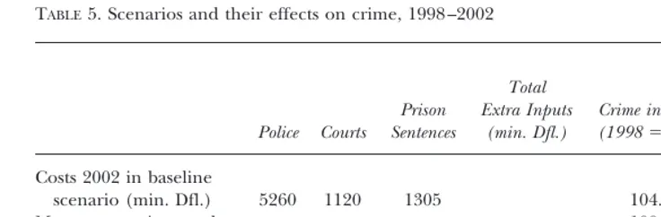
VII. Simulations
Combining the various parts of the model enables us to sketch possible scenarios of crime and punishment in the near future. It also enables us to estimate the cost-effectiveness, in terms of reductions in crime, of spending extra money in different parts of the law enforcement system. Table 5 presents the results of five scenarios over the period 1996 to 2002. The first scenario (the baseline scenario) assumes that economic growth will be modest, in line with the lower estimate of the Dutch Central
Planning Bureau. Demographic forecasts are based on the medium forecast of the Dutch Central Bureau of Statistics. The second scenario assumes a more optimistic economic trend (with income distribution remaining equal).
The third, fourth, and fifth scenarios are, compared with the baseline scenario, all based on an increase in expenditure by 100 million Dutch guilders in two parts of the law enforcement system. In the first law enforcement scenario, extra money is spent mainly on police to increase the clear-up rates. In this scenario, extra inputs into courts and prisons are only meant to keep the probability and length of imprisonment constant. In the second scenario, the courts get extra money to increase the probability of punishment and imprisonment. To keep the average length of imprisonment con-stant, the inputs into the prison system have also to increase. In the third law enforce-ment scenario, only the probability and length of imprisonenforce-ment are increased. There-fore, extra money is spent on the prison system.
In the baseline scenario, the number of crimes will rise by 4.9% in the period 1998 to 2002. According to our model, economic trends have a considerable impact on this result. A more favorable scenario of economic growth leads to a stabilization of crime rates. Within the three scenarios that provide for extra inputs into the law enforcement system, increasing the prison sentences is shown to be the most effective.
At first sight this is surprising, because the elasticity of crime related to the clear-up rate is greater than that related to the probability of being imprisoned or the length of imprisonment (see Table 1). So, increasing the clear-up rate is potentially a useful policy to reduce crime. But simply increasing police inputs is not very cost effective because of two reasons: (1) the effects on the clear-up rate are relatively modest (see Table 3); and (2) as a consequence of rising clear-ups, not only police inputs but also inputs into courts and prisons have to rise to keep imprisonment rates constant.
Obviously, these results give only rough indications. They show the impact of auton-omous social factors on crime rates and the relatively limited influence that law en-forcement has. They are further limited in the sense that other policies, such as social prevention measures or improvements to law enforcement efficiency, have not been considered.
VIII. Conclusions
This article presents a preliminary version of a macroeconomic model of the Dutch criminal justice system for the period 1957 to 1995. The model links together the TABLE5. Scenarios and their effects on crime, 1998 –2002
Police Courts
scenario (min. Dfl.) 5260 1120 1305 104.9
More economic growth 100.8 24
Extra police 93 0 7 100 104.9 20.06
Extra courts 0 84 16 100 104.9 20.02
Extra prisons (sentences) 0 0 100 100 103.4 21.43
number of crimes, the responses of the criminal justice system, and the inputs into that system by econometric estimations. The estimations are then used to sketch some scenarios.
The model consists of four parts:
1. The number of crimes of various types of crime is linked to demographic, social, and economic factors on one side and to law enforcement characteristics, like the probability and severity of punishment, on the other side.
2. The number of crimes cleared up by the police is linked to the number of recorded crimes, the inputs into the police, and time-trends.
3. The number of guilty verdicts by the courts (including the public prosecutions departments) is linked to the number of cases handled (which is linked to the number of crimes cleared up), the inputs into the courts, and time-trends. 4. The proportion and length of prison sentences are estimated by pure time-series
analysis. No clear explanatory factors could be found here.
The empirical estimations show that both demographic, social, and economic factors and the results of the law enforcement system influence the number of crimes. For violence, petty thefts, and other crimes, a rise in the clear-up rate reduces the crime rate. The average term of imprisonment has a negative impact on violence. A growth in the number of young men, divorced persons, unemployed, drug addicts and motor vehicles— each per capita—and a rise in income inequalities have a boosting effect on one or more types of crime.
Recorded crimes have more impact on the police output than the total volume of inputs. The time-trend effects are generally negative and are more strongly so in the second half of the period.
Just like the police output, the outputs of the public prosecutions department and the judicial system are more affected by the number of handled cases (see recorded crimes for the police) than by the total volume of inputs.
The scenarios presented here show the impact of economic trends on crime rates. Different scenarios of spending extra money in the law enforcement system give clear and interesting differences. Raising the length of prison sentences seems more cost-effective than increasing the inputs into police, public prosecutors departments, and courts. This is because simply spending more money on police or courts is not very cost effective for two reasons: (1) The effects on the clear-up rate and punishments respec-tively are relarespec-tively modest; and (2) as a consequence of rising clear-ups or punishments, not only police and court inputs have to rise but also inputs into the latter parts of the law enforcement chain.
We have illustrated in this way the potential use of this type of model for policy purposes. It is clear that the model presented here can be extended and improved. The use of macroeconometric time-series analysis has clearly its limitations. In the future, we hope to be able to enrich the model with further analyses, for example, in the sphere of cross-section analysis at the microeconomic level.
Appendix
The actual estimated model is as follows (error terms have been omitted)
1b1iDln
Po 5size of the total population
Upi 5number of clear-ups of type i (i51...,6)
Cai 5number of settled cases by the public prosecutor or the court of
different types of crime (i51...,6) (strong correlation with the num-ber of clear-ups)
Pui 5number of punishments of different types of crime (i51...,6)
Imi 5number of imprisonments of different types of crime (i51...,6)
Imij 5number of imprisonments of different types of crime and different
terms (i51...,6 and j51,...,5)
Ti 5average term of imprisonment of different types of crime (i51...,6)
XP 5total volume of police inputs (labour and material, measured as de-flated costs)
XJ 5total volume of inputs of the administration of justice (labor and material, measured as deflated costs)
Yo 5number of young men
Di 5number of divorced
NN 5number of non-natives
Un 5number of unemployed and incapacitated
Inc 5average disposable income
Th 5Theil-coefficient
Dr 5number of clinic admissions of drug addicts
Mo 5number of motor vehicles
Greek letters 5constants to estimate
References
BECKER, G.S. (1968). “Crime and Punishment: An Economic Approach.” Journal of Political Economy
76:169 –217.
BLOCK, MICHAELK.,ANDTHOMASS. ULEN. (1979). “Cost Functions for Correctional Institutions.” InThe Costs of Crime, ed. Charles M. Gray. Beverly Hills, CA: Sage Publishers.
CARR-HILL, R.A.,ANDN.H. STERN. (1979).Crime, the Police and Criminal Statistics. An Analysis of Official Statistics for England and Wales Using Econometric Models. London: Academic Press.
DARROUGH, M.N.,ANDJ.M. HEINEKE. (1978). “The Multi-Output Translog Production Cost Function: The Case of Law Enforcement Agencies.” In Economic Models of Criminal Behaviour, Contributions to Economic Analysis series no. 118, ed. J.M. Heineke. Amsterdam: North-Holland Publishing Com-pany.
DARROUGH, M.N.,ANDJ.M. HEINEKE. (1979). “Law Enforcement Agencies as Multi-Product Firms: An Econometric Investigation of Production Costs.Public Finance34:176 –195.
EIDE, ERLING. (forthcoming). ”Economics of Criminal Behavior.“ InEncyclopedia of Law and Economics, eds. B. Bouckaert and G. de Geest. Aldershot, U.K.: Edward Elgar.
GANLEY, JOE,ANDJOHNCUBBIN. (1987). ”Performance Indicators for Prisons.“Public MoneyDecember:
57–59.
GANLEY, J.A.,ANDJ.S. CUBBIN. (1992).Public Sector Efficiency Measurement: Applications of Data Envelopment Analysis. Amsterdam: North Holland.
GILLESPIE, ROBERTW. (1976). ”The Production of Court Services: An Analysis of Scale Effects and Other Factors.“Journal of Legal Studies5:243–264.
GOUDRIAAN, R., F.VANTULDER, J. BLANK, A.VAN DERTORRE,ANDB. KUHRY. (1989).Doelmatig dienstverlenen. Rijswijk/Alphen aan den Rijn, Social and Cultural Studies series, no. 11. The Netherlands: Social and Cultural Planning Office/Samson.
GOUDRIAAN, RENE´,ANDFRANK VANTULDER. (1993). ”Scale and Efficiency of Police Departments.“ Paper prepared for the XXXVIIIth International Conference of the Applied Econometrics Association, Athens, Greece, April, 1993.
GYIMAH-BREMPONG, K. (1989). ”Demand for Factors of Production in Municipal Police Departments.“ Journal of Urban Economics25:247–259.
HAYES, ROBERTD.,ANDJAMESA. MILLAR. (1990). ”Measuring Production Efficiency in a Not-For-Profit Setting.“The Accounting Review65:505–519.
HAYES, ROBERTD.,ANDJAMESA. MILLAR. (1993). ”A Rejoinder to ’Measuring Production Efficiency in a Not-For-Profit Setting: An Extension.’ “The Accounting Review68:89 –92.
KITTELSEN, SVERREA.C.,ANDFINNR. FOERSUND. (1992). ”Efficiency Analysis of Norwegian District Courts. The Journal of Productivity Analysis3:277–306.
LEWIN, ARIEY., RICHARDC. MOREY,ANDTHOMASJ. COOK. (1982). “Evaluating the Administrative Effi-ciency of Courts.”OMEGA10:401– 411.
MENSAH, YAW M., AND SHU-HSING LI. (1993). “Measuring Production Efficiency in a Not-For-Profit Setting: An Extension.The Accounting Review68:66 – 88.
PHILLIPS, LLAD,ANDHAROLDL. VOTEY, JR. (1981).The Economics of Crime Control, Sage Library of Social Research, Vol. 132. Beverly Hills, CA: Sage Publications, Inc.
SHINNAR, R.,ANDS. SHINNAR. (1975). ”The Effects of the Criminal Justice System on the Control of Crime: A Quantitative Approach.“Law and Society Review9:581– 611.
TULKENS, HENRY. (1990). ”Non-Parametric Efficiency Analysis in Four Service Activities: Retail Banking, Municipalities, Courts and Urban Transit,“ CORE-discussion paper no.9050. Louvain-la-Neuve, France: Center for Operation Research and Econometrics.
VAN TULDER, FRANK. (1993). ”Law Enforcement, Production and the Decision-Making Process: An Analysis of Dutch Police-Departments.“ Paper presented at the 49th IIPF-Congress on Public Finance and Irregular Activities.
VANTULDER, F. (1994).Van misdaad tot straf, Social and Cultural Studies series no.21. Rijswijk/The Hague: Social and Cultural Planning Office/VUGA (thesis with English summary).
WELLER, DENNIS,ANDMICHAELK. BLOCK. (1979). ”Estimating the Cost of Judicial Services.“ InThe Costs of Crime, ed. Charles M. Gray. Beverly Hills, CA: Sage Publications.