q
Research supported by the Natural Sciences and Engineer-ing Research Council of Canada.
1Present Address: School of Operations Research & Industrial Engineering, Cornell University, Ithaca, NY 14858, USA.
*Corresponding author. Tel.:#1-519-888-4567; fax:# 1-519-746-7252.
E-mail address:[email protected] (Y. Gerchak).
Continuous review inventory models where random lead time
depends on lot size and reserved capacity
qMetin C
7
akanyildirim
1
, James H. Bookbinder, Yigal Gerchak*
Department of Management Sciences, University of Waterloo, Waterloo, Ont., Canada N2L 3G1
Received 6 April 1998; accepted 2 August 1999
Abstract
The processing time of large orders is, in many industries, longer than that of small orders. This renders supply lead times in such settings to be increasing in the order size. Yet that pattern is not re#ected in existing inventory control models, especially those allowing for random lead times. This work aims at rectifying the situation. Our setting is an order-quantity/reorder-point model with backordering, where the shortage penalty is incurred per unit per unit time. The processing time of each unit is random; the processing time of a lot is correlated with its size. For the case where lead time is proportional to the lot size, we obtain a closed-form solution. That is, unlike the classical (Q,r) model (where lead time is independent of lot size), no iterations are required here. We also analyze a case where the processing time exhibits economies of scale in the lot size. Finally, we consider a situation where a customer can secure shorter processing times by reserving capacity at the supplier's manufacturing facility. ( 2000 Elsevier Science B.V. All rights reserved.
Keywords: Inventory control; Continuous review; Random lead time
1. Introduction
The goal of this work is to explore the implica-tions, in a continuous review inventory model, of
randomlead times being contingent on lot size. It is
motivated by the rather obvious observation that manufacturing larger lots often requires longer time. While waiting time and machine setup time
are usually independent of lot size, the actual processing-time portion of lead time could well depend on the lot size in many industries which manufacture discrete parts or products. Yet exist-ing inventory control literature (e.g. [1}3]) does not explicitly incorporate lot-size dependency into the way it models lead times. We aim at rectifying this situation.
Someindirectimplications of replenishment
pol-icies for supply lead times have been investigated before. In references on multiple sourcing when lead times are random (e.g. [4]), order splitting among several suppliers causes one of the orders to tend to arrive earlier than had there been a single supplier, thereby reducing e!ective lead time. Selecting suppliers by the length and/or variability of their lead times has been explored by Gerchak
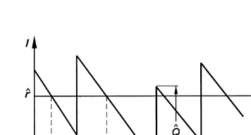
Fig. 1. The installation stock in the backorder case. LT stands for lead time.
and Parlar [5], Choi [6] and Bookbinder and
C7akanyildirim [7]. But neither strand of the
litera-ture allowed a given supplier's lead time to be dependent on (i.e. increasing in) the lot size.
Our setting is a (Q,r)
order-quantity/reorder-point model withbackordering, where the shortage
penalty is incurred per unit per unit time. Demand rate is assumed constant, while the lead-time is random. In line with most researchers, we assume that immediately after the arrival of an order the installation stock will always exceed the reorder level, so at most one order will be out-standing at any time. The processing time of
a single-unit order is a random variable, ¹; the
processing time of a lot ofQunits is assumed to be
a multiple of¹,Qh¹, where the value of the positive
parameter hindicates the extent of economies of
scale and/or learning e!ects, if any, in production
speed. We focus speci"cally on the values h"1
(no economies of scale) and h"1/2 (positive
economies).
For the case h"1, in Section 3 we prove joint
convexity in (Q,r) and obtain closed-form
expres-sionsfor the decision variables. Thus, as opposed to
the classical lot-size-independent lead-time model
(which might be viewed as corresponding toh"0
in our setting), our`linearamodel doesnotrequire
an iterative procedure for obtaining the solution.
The case h"1/2 is more complicated to analyze;
there we establish joint convexity within a certain range. An example (Section 4) is then used to show that the joint-convexity range may indeed be large enough to guarantee global optimality of the solu-tion to the necessary condisolu-tions. That solusolu-tion, however, must be obtained in an iterative fashion, which we illustrate. Numerical examples are
pre-sented in Section 5, comparing solutions forh"1
and 1/2 and conducting some sensitivity analyses with respect to the cost parameters.
In the previously described models, the time needed to produce a single item was assumed to be
an exogenous random variable. Our "nal model
relaxes this assumption in Section 6 via the use of
reserved capacity. The idea of using supply
con-tracts which`reserveacapacity at the supplier for
a particular customer, thereby ensuring timely sup-ply, appears to be growing in popularity, and has recently been explored by several researchers,
in-cluding Karmarkar et al. [8], Silver and Jain [9], Jain and Silver [10] and Anupindi and Bassok [11]. Our model assumes that the capacity avail-able for a particular order is the sum of the reserved production rate and an additional random rate (which will depend on the supplier's situation at the moment). A single item's processing time is then assumed to be the reciprocal of that sum of capaci-ties. Random capacity was previously envisioned as restricting output quantity [12}14]. We, on the other hand, view it as a factor in determining the lead time.
For any level of reserved capacity, one can"nd
the best values ofQandrusing the methods
out-lined earlier. A search for the optimal capacity to reserve is then conducted. We outline a procedure, but leave the detailed investigation of this model for future research.
2. The model and its properties
Production costs are not explicitly included, since all demand is eventually met. An inventory
holding cost ofhK per unit per unit time is assumed,
and a "xed cost of K is incurred for each order
placed. Also, a shortage cost ofn( per unit per unit
time is incurred when a demand is backlogged. For reasons that will become clear, let us for the
mo-ment denote by QK and r( the order quantity and
reorder point.
Let g be the probability density of lead time.
shortage costs per cycle can be computed as
We shall now scale the constant demand rate to
unity; the decision variables QK and r( will then be
expressed in units of time rather than quantity. For
illustration, suppose thatD"10 packets per day,
QK"50 packets,r("20 packets. We may scale de-mand to unity by visualizing a single day's dede-mand
(10 packets) as one quantity-unit. LetQandr
de-noteQK andr(, respectively, after scaling, thenQ"5
days'demand andr"2 days'demand. In general,
Qwill beQK/Dday's demand andrwill ber(/Ddays'
demand. Thus the dimensions ofQandrare time,
not quantity any more.
To maintain accuracy in the costs, we have to
scale them as well. Lettinghandnbe the costs after
scaling, we have h"DhK and n"Dn(. The scaled
holding and shortages costs per cycle are then
!h
P
rThus by the renewal reward theorem (e.g. [15]), the expected cost per unit time is
EMC(Q,r)N"
G
K!hP
rsizeQis assumed to equal
¸(Q)"Qh¹, h*0,
where¹is the processing time of a single-unit lot.
Clearly,¸(Q) is stochastically increasing inQ.
Let G denote the distribution function of lead
time.Gandgcan respectively be expressed in terms
of the distributionFand probability density
func-tionfof the processing time¹of a single-unit lot, as
follows:
Substituting in terms of the distribution of ¹, we
have
This completes our formulation of the problem. Before discussing convexity properties and solu-tion algorithms, let us make the following remarks.
neglected the portiont
0 of lead time that is
inde-pendent ofQ. The total lead time is thust
0#¸(Q),
where t
0 includes allowances for materials
hand-ling, waiting and setup. Although t
0 will often be
the major component of total lead time, there are
many circumstances wheret
0can be approximated
as constant, independent of the random variable¹.
Bookbinder and C7akanyildirim [7] then show that
m(x), the probability density function of lead time,
accounting fort
0, is a shift to the right byt0in the
lead-time densityg(x) pertinent to only the portion
¸(Q). They found therefore that the optimalQwas
una!ected by the shift, whilerwas simply increased
by t
0. This is why, in the present paper, we have
concerned ourselves with just the¸(Q)-segment of
lead time.
Returning now to"nding the optimal pair (Q,r)
for objective function (3), one seeks critical points of
the expected-cost function overM(Q,r)3R2:Q*0,
r*0N. Such a search will converge to the global
minimum if joint convexity of (3) can be proven. First, however, we shall study convexity of that
portion ofEMC(Q,r)Ncorresponding to the expected
number of units backordered. It is worth mention-ing that Zipkin [16] proved convexity of this func-tion for a lot-size-independent lead time.
Letting y"x/Qhin (3), the expected number of
units backordered is given by
B(Q,r)"
P
=Proposition 1. For h"1, the expected number of
units backordered is jointly convex in(Q,r).
Proof. Taking second partial derivatives of the
functionB(Q,r), the Hessian matrix is found to be
H"
A
r2(1!F(r/Q))/Q3 !r(1!F(r/Q))/Q2 !r(1!F(r/Q))/Q2 (1!F(r/Q))/QB
.(5)
Since the term 1!F(r/Q) is non-negative, and
the determinant of the Hessian matrix is zero, the
Hessian is positive semide"nite (e.g. [17]). Hence, the expected-units-backordered cost function is
jointly convex. h
To help us analyze the case h"1/2, we let
d"r/Qh, so
B(Q,d)"Q2h~1
P
=y/d
(y!d)2f(y) dy/2. (6)
Proposition 2. If h"1/2, the expected number of
units backordered is jointly convex in(Q,d).
Proof. For that value ofh,B(Q,d) reduces to
B(d)"
P
=y/d
(y!d)2f(y) dy/2. (7)
Thus convexity reduces to showing that the second
derivative of (7) with respect todis positive, which
is immediate. h
We have so far proved convexity of the expected number of units backordered. To consider
convex-ity of the entire objective function, let k"E(¹).
The objective (3) takes the following form when
h"1:
EMC(Q,r)N"K/Q#(n#h)B(Q,r)
#h(r#Q/2!kQ). (8)
Using Proposition 1, it is easy to show:
Corollary 1. Forh"1,the expected-cost function(8)
is jointly convex in(Q,r).
By similar arguments, the objective function for
h"1/2 turns out to be
EMC(Q,d)N"K/Q#(n#h)B(d)
#h(dQ1@2#Q/2!kQ1@2). (9)
Looking at (9), term by term, in conjunction with Proposition 2, reveals that all terms are always
convex ind, and are convex inQifd)k. Hence we
Corollary 2. Forh"1/2,the expected-cost function
is convex ind,and, ifd)k,it is also convex inQ.
We now examine the Hessian of total expected
cost forh"1/2. After some algebra, that Hessian
turns out to equal
A
(n#h)(1!F(d)) h/2Q1@2h/2Q1@2 2K/Q3#(k!d)h/4Q3@2
B
. (10)Without substituting the optimality conditions, it is not easy to show positive de"niteness of (10). We therefore defer this discussion to Section 4, where we obtain the critical points for concave
processing time. Let us "rst study the necessary
conditions whenh"1.
3. Critical points for linearly varying processing time
Since we established the convexity of expected costs, critical points of the objective function (8) will be global minimizers. Proposition 3 characterizes
those points through"rst-order optimality
condi-tions for Q and r. The proof follows directly by
di!erentiating the function, plus some algebra.
Proposition 3. The optimality conditions are
P
=At "rst glance, both (11) and (12) appear to be
functions of Qand r, and iterating between these
two conditions would thus be unavoidable. How-ever, an important observation eliminates the need
for iterative solutions. Let us refer tod"r/Qas the
`single-unit reorder pointa, since dis the optimal
reorder level when the lot size is one. The
optimal-ity conditions become
Then, minimization of expected costs can be achieved via the following algorithm:
1. Solve (13) for the single-unit reorder point,d.
2. Calculate the lot size,Q, by solution of (14).
3. The reorder point isr"Qd.
In contrast to solving for the optimal values of
Q and r in the classical (Q,r) model (e.g. [18]),
corresponding toh"0 in our general model, we
obtained here (when h"1) a one-pass procedure
(not requiring iterations) to "nd the decision
variables.
It is easy to see that the single-unit reorder point
dincreases with the shortage costnand decreases
with the holding costh, and that the optimal lot size
Qincreases in the setup costK.
Let us illustrate our"ndings by specializing to
exponential single-unit processing time.
Example 1. Suppose
f(t)"jexp(!jt), t*0. (15)
Note that E(¹) must be less than one, i.e.j'1;
otherwise, in the long run, the production rate will not su$ce to meet demand. For this density (15), the expected-cost expression becomes
EMC(Q,r)N"K/Q#(n#h)QMexp(!jr/Q)N/j2
#h(r#Q/2!Q/j). (16)
We thus obtain the following solution:
d"!Mln[hj/(n#h)]N/j, (17)
Q2"2K/h(2d#1). (18)
Eqs. (17) and (18) reveal that Q decreases in n,
4. Critical points for concave processing time (h51/2)
Concave processing time appears to be more plausible in practice than linear processing time. Having already discussed convexity and estab-lished the necessary conditions in Corollary 2, we shall next investigate the critical points of (9). Prop-osition 4 will directly provide the optimality
condi-tions forQandd. (dis still the`single-unit reorder
pointa, sinced"r/Q1@2 remains the optimal
reor-der level whenQ"1.)
Proposition 4. The optimality conditions are
P
= y/d(y!d)f(y) dy"hQ1@2/(n#h), (19)
Q2#(d!k)Q3@2!2K/h"0. (20)
Proof. Eqs. (19) and (20) follow by di!erentiating
(9) with respect todandQ, respectively, and setting
each equal to zero. h
Returning to the issue of the joint convexity of (9), our"rst result is
Proposition 5. The second derivative of the
expected-cost function with respect to Q is positive
whereQis critical,i.e. where(20)is satisxed.
Proof. From (10), this second derivative equals
2K/Q3#(k!d)h/4Q3@2. (21)
It follows that (21) is positive if and only if
8K/h#(k!d)Q3@2 (22)
is positive. This is clearly so for any Qsatisfying
(20). h
Corollary 2 implies that the expected costs are
convex for din a certain range, whereas
Proposi-tion 5 says that the expected costs are convex at
criticalQvalues over all values ofd. We now assert
the joint convexity of the expected costs.
Proposition 6. If d)F~1Mn/(n#h)N, the Hessian
(10)is positive dexnite at critical points Q.
Proof. We need to show only that the determinant
of (10) is positive at critical values ofQ and over
dsatisfying the above condition. That determinant
equals
(n#h)(1!F(d))M(k!d)h/4Q3@2#2K/Q3N!h2/4Q
"M(n#h)(1!F(d))((k!d)hQ3@2#8K)
!h2Q2N/4Q3. (23)
Next substitute Q2h!2K for (k!d)hQ3@2, since
Qsatis"es (20). After some algebra, we"nd that (23)
is positive if and only if
n!(n#h)F(d)#6Kh/(6K#Q2h)*0, (24)
which is always true for the given range ofd. h
We shall henceforth denote by A the region
M(Q, d)3R2:Q'0, 0(d)F~1(n/(n#h))N. Proposition 6 is important in the sense that it
guarantees joint convexity at a critical pointQfor
any d in A. Solution of (19) and (20) thus yields
a local minimum if (Q,d)3A. Recall, however, that
a di!erentiable function, convex at all its critical points in a region, can have at most one minimizer
there. Thus if (Q,d)3Afor some critical Qand d,
then this point is a global minimizer inA. So the
larger the rangeA, the more likely it is that a
solu-tion of (19) and (20) will yield the real minimizer
*the global one. As our examples will reveal, that
range is large enough for reasonable problem parameters.
Unlike the optimality condition (13), Eq. (19)
does depend onQ, hence we cannot avoid an
iter-ative solution scheme. We apply coordinate descent (e.g. [17]) to obtain the critical points of (9). Our method is outlined below.
0. InitializeQ"EOQ.
1. GivenQ, solve fordin (19).
2. With thatd, obtainQvia (20).
3. Return to Step 1 unlessQdoes not di!er much
from its previous value.
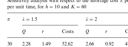
Table 2
Values of objective function (16) (h"1) and global minimizers. Sensitivity analysis with respect to the shortage costnper unit per unit time, forh"10 andK"60
n j"1.5 j"2
Q r Costs Q r Costs
30 2.28 1.49 52.62 2.66 0.92 45.07
45 2.10 1.81 57.26 2.44 1.23 49.13
60 1.98 2.04 60.54 2.31 1.45 51.99
Table 1
Minimum expected costs and optimal decision variables with variation inK, the setup cost per order, whenh"1,h"10,
n"30
K j"1.5 j"2
Q r Costs Q r Costs
40 1.86 1.22 42.97 2.17 0.75 36.80
50 2.08 1.36 48.04 2.43 0.84 41.15
60 2.28 1.49 52.62 2.66 0.92 45.07
It is known that all coordinate-descent algo-rithms, minimizing a function with unique min-imum along any coordinate direction, converge [17]. By Corollary 2, the expected costs are such
a function for d)k. Therefore, over the region
MQ*0, 0)d)kN, our algorithm converges to the
pair (Q,d) which simultaneously solves (19) and
(20). Outside that region, convergence cannot be guaranteed.
Another issue is whether solving (19) and (20) indeed yields minimizers, as opposed to maximizers or saddle points. It is clear from Corollary 2 that the expected-cost function cannot be concave. Critical points are thus not maximizers, although
they may be saddle points if (Q,d)NA. Therefore, to
establish convexity outside the regionA, it is
neces-sary to evaluate the Hessian. To illustrate, let us
again specialize to exponential single-unit
processing time, as in Example 1.
Example 2. The expected costs will now equal
EMC(Q,r)N"K/Q#(n#h)Mexp(!jd)N/j2
#h(dQ1@2#Q/2!Q1@2/j). (25)
The optimality equations given in (19) and (20) respectively reduce to
d"!Mln(hjQ1@2/(n#h))N/j, (26)
Q2#(d!1/j)Q3@2!2K/h"0. (27)
We now eliminatedfrom (27) by inserting (26) to
obtain
Q2!Mln(hjQ1@2/(n#h))#Q3@2N/j!2K/h"0. (28)
Eq. (28) can be solved numerically for Q. For
example, if j"2, h"10, n"40 andK"50, we
obtainQ"3.513. The correspondingdturns out to
equal 0.144. (Note that sinced(k"1/2, an
iter-ative coordinate descent would have converged here).
For the exponential density, the su$cient condi-tion of Proposicondi-tion 6 becomes
exp(!jd)*h/(n#h). (29)
From (26), it is clear that (29) holds as long as
jQ1@2*1. Hence if processing time is exponential,
there is a large range ofdfor which expected costs
will be jointly convex.
5. Numerical examples
In this section, we again assume an exponential
distribution for the time ¹ to produce one unit,
thereby extending Examples 1 and 2. We shall
examine changes in the optimal lot size Q and
reorder point r as the cost parameters vary, for
both the linear and concave models.
5.1. h"1
Tables 1}3 illustrate results when lead time
de-pendslinearlyonQ.
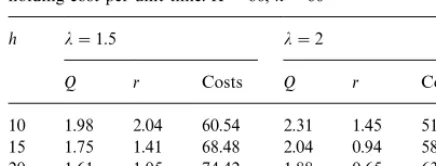
Table 3
Minimum expected costs (16) and optimal (Q,r) as we varyh, the holding cost per unit time.K"60,n"60
h j"1.5 j"2
Q r Costs Q r Costs
10 1.98 2.04 60.54 2.31 1.45 51.99
15 1.75 1.41 68.48 2.04 0.94 58.73
20 1.61 1.05 74.42 1.88 0.65 63.75
2We wish to thank Ton de Kok and S+ren Glud Johansen for proposing this idea.
Consider two inventory managers,AandB, both
with a cost structureK"40, h"10 andn"30. In
each case, the true relationship is that lead time
depends linearly onQand the single-unit lead time
is exponential with meank"2/3. ManagerA
rec-ognizes the dependences of lead time on lot size.
She thus"nds, from the"rst row of Table 1, that
Q"1.86 and r"1.22, for a (minimum) cost/unit
time of$42.97.
ManagerB, however, employs the classical (Q,r)
model; he overlooks the relationship ¸(Q).
Sup-pose, in the"rst instance,Btakes the lead-time for
the entire lot as exponentially distributed with
mean 2/3. He will then obtainQ"3.34 andr"0,
incurring a cost per unit time of$66.53, 54% above
that ofA.
Now suppose that Manager A tells B that she
calculated the optimal lot size as 1.86, which made the expected lot lead time be 1.24. If Manager
Btakes lead time as exponential, but still
indepen-dent of lot size, with mean 1.24, he will end up with (Q"4.33,r"0.17) and an inventory cost of$76.30
per unit time, 77% higher than what A incurs.
Comparing his cost performance to A's, B may
think that he wrongly anticipated short lead times.
Hence,Bmay assume a stochastically longer lead
time, say with expected value of 2.28 (twice the
whole lot lead timeAexperiences). ThenBwill"nd
(Q"6.24,r"1.15), incurring$91.70 per unit time,
now 113% more thanA's cost.
It is worth noting that B, failing to realize the
dependence of lead time on lot size, tended to choose larger lot sizes, hence faced longer lead times than he would have thought. Not
appreciat-ing the lot-size dependence also causedBto incur
excess costs.
Suppose now that managerCemploys the
classi-cal (Q,r) model (with per-unit-time shortage
pen-alty), but the lead-time distribution used in each step of the iterations is the one corresponding to the
current value of Q. (Iterations would begin with
Q"EOQ, perhaps as in the model allowing
short-ages.) ThusC recognizes the correct form of lead
time's dependence on the lot size, but does so with-in optimality equations derived from a model which ignores such dependence.2
If lead-time distribution is exponential, then the expected number of units backordered is
n(r)"e~jr/j.
The optimality conditions become
Q"J2(K#ne~jr/j2)/h, e~jr/j"Qh/n.
Thus
Q"1/j#J1/j2#2K/h
and
r"!ln[h(1#J1#2j2K/h)/n]/j.
Since from the above
j"Q/(Q2/2!K/h),
that will be the (reciprocal of the) mean lead-time
for a particularQ.
We looked at some numerical examples and the costs turned out to be very high relative to the
optimal costs. We feel, however, that this
conclusion may be rather meaningless, since the models are not really comparable; the lead-time distribution, which is here consequential, cannot be made identical with an externally hypothesized
distribution of¹inQ¹.
5.2. h"1/2
Tables 4}6 show how the optimal Q and r
Table 4
Minimum expected costs and optimal decision variables with variation in K, the setup cost per order, when h"1/2, h"10,n"30
K j"1.5 j"2
Q r Costs Q r Costs
40 3.21 0.47 33.26 3.26 0.09 29.49
50 3.61 0.43 36.19 3.65 0.04 32.39
60 3.97 0.39 38.83 4.00 0.00! 35.00
!The optimal (unrounded)requals zero.
Table 5
Values of objective function (25) (h"1/2) and global minim-izers. Sensitivity analysis with respect to the shortage costnper unit per unit time, forh"10 andK"60
n j"1.5 j"2
Q r Costs Q r Costs
30 3.97 0.39 38.83 4.00 0.00! 35.00
45 3.67 0.83 42.99 3.80 0.34 38.14
60 3.52 1.14 46.04 3.66 0.58 40.47
!The optimal (unrounded)requals zero.
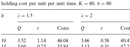
Table 6
Minimum expected costs (25) and optimal (Q,r) as we varyh, the holding cost per unit per unit time.K"60,n"60
h j"1.5 j"2
Q r Costs Q r Costs
10 3.52 1.14 46.04 3.66 0.58 40.47
15 3.04 0.75 53.84 3.13 0.31 47.23
20 2.76 0.52 59.82 2.28 0.15 52.41
time isconcavein lot size. Note in these tables that
jQ1@2*1, so the expected cost is jointly convex at
the pointsQandrlisted below.
5.3. Discussion
For both cases (linear and concave), the changes in optimal values of the decision variables can be
summarized as follows:
(a) Qincreases inK, and decreases innandh.
(b) rincreases inn, but decreases inh.
These observations are intuitive [cf. comparative
statics for the classical (Q,r) model with
time-inde-pendent shortage penalty in [19]].
The impact of the setup costK on the reorder
pointris, however, interesting. In the
linear-lead-time case,r increases in K (Table 1), whereas for
concave lead timerdecreases inK. This could be
explained as follows. Eq. (13) reveals that in the linear model, the optimal single-unit reorder point
dis actually independent of the setup costK. Since
the optimal ris a product of d and Q, andQ
in-creases inK, so doesr. On the other hand, in the
concave modelddecreases inQEq. (19), so when
K rises, Q increases and d decreases. Thus the
direction of change inr"Q1@2dis not clear.
Appar-ently, in our examples, the decline indwas great
enough to compensate for the rise in the lot sizeQ,
causing the reorder pointrto go down.
Another way to explain the preceding is that,
when ¸(Q)"Q1@2¹, increasing Q economizes on
setups and reduces the average lead time per unit. When the average lead time per unit decreases, it is plausible that the reorder point also does.
One could interpret the parameter j as
a measure of capacity. It is noteworthy that by
augmentingjfrom 1.5 to 2 in each of Tables 1}6,
the total costs decrease in every row. Therefore, it is quite reasonable to look for ways to increase capacity permanently, even at some expense.
6. Lot-size-dependent lead time under reserved production rate
Until now, we assumed that the stochastic lead
time¹to produce one unit was independent of the
decision variables; in other words, it wasexogenous.
In this section, that duration will be made an
endo-genousrandom variable by establishing a link
We envision the lead time to be inversely related to capacity. The capacity allocated to a particular
order consists of an amountadedicated
(contrac-ted-for) to that customer, and a random portionC,
which depends on congestion at the moment and commitments to other customers. Thus
¸(Q)"Qh/(a#C).
SupposeChas distribution functionH. It follows
that the lead-time distribution, which we still
denote by G, depends on that of Cvia
G
Q(x)"PMQh/(a#C))xN
"P(C*Qh/x!a)"HM (Qh/x!a). (30)
To obtain the expected inventory costs for a given
a, begin by putting (2) in the form
Let us henceforth restrict attention to the case
h"1. If one substitutes (30) in the expected costs,
keeping in mind that lead time cannot exceedQ/a,
we get
Due to the upper bound on lead time, the reorder
point satis"esr(Q/a. Otherwise, the holding costs
could be reduced by lowering the reorder level without altering other costs.
To complete the expected-cost expression, we must include the costs to reserve a production
capacitya. A customer may have to compensate the
manufacturer for dedicating this capacity to its
exclusive use. Such an expense arises because the manufacturer distorts its production process, per-haps incurs overtime or hires extra workers, or pays a tardiness penalty to some other customers. The cost to reserve a production rate can be charged to the customer in one of the two ways: either on the basis of cost per unit quantity or cost per unit time (cf. [5]). However, since demand was scaled to be one unit per time period, it does not formally matter how we model the cost to reserve the rate; expected-cost expressions will be the same in both cases.
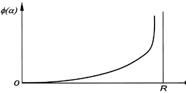
Although the upper level of reserved production could, in principle, be the manufacturer's total
production rate R, a customer would be charged
excessively to bring its reserved rate so high. Reser-vation costs will thus be convex; a possible shape
/(a), to reserve the production ratea, is in Fig. 2.
If /(a) is added to the previous expected-cost
expression (32), with the reserved production rate
aa third decision variable, the objective function
becomes
that, for a"xed reserved capacitya, Eq. (33) reduces
to (3) withh"1. Thus, all convexity and"rst-order
optimality results are still valid, i.e. (33) is jointly
convex inQandr, and closed-form expressions are
available for the minimizers. What we need then is
a mechanism to"nd theawhich minimizes (33) for
"xedQandr; we shall again employ a coordinate-descent-based algorithm. By di!erentiating (33)
with respect toa, we obtain the following equation
whose solutions are critical values ofa:
Fig. 2. Cost of reserving a production ratea.
Fig. 3. Illustration of the steps of the algorithm.
Therefore, we propose in Fig. 3 an algorithm to"nd
optimal values of the decision variables.
That algorithm starts by"ndingQandd"r/Q
for"xeda. This is Step 1, and we have already given the closed-form results for that in Section 3. Step
2 is basically solution of Eq. (34) whenQandrare
given. Step 1 is extremely simple, so Step 2 (solving a nonlinear equation) dictates the level of e!ort. We note that one has to check for joint convexity by evaluating numerically the Hessian at critical points, before concluding that the result is really a minimizer.
7. Conclusions
This paper modeled, and explored the implica-tions of, dependence of random lead time on lot size and production capacity. We discussed mainly two cases: lead time linear and concave in lot size. Joint convexity of expected costs was established in the
decision variables Qand r. First-order conditions
for Qand rwere laid out, and (for h"1)
closed-form results for optimal decision variables were obtained from those conditions. Numerical exam-ples and sensitivity analyses on cost parameters were provided for both models. A comparison of the way linear and concave lead-time models re-spond to cost parameters was presented.
Reserving some of a manufacturer's production capacity was then examined. Orders were assumed
to be allocated the sum of the reserved and random
capacity. The reserved capacity, a, then became
a decision variable, in addition toQandr. Since for
"xed reserved capacity this model reduces to the one discussed earlier in the paper, many results carried over automatically. Indeed, the di$cult part was solving the nonlinear optimality equation
fora, givenQandr. Some of this was left for future
work.
The models presented here might be extended in the following ways. Our results pertaining to a backordering situation could serve as the basis for analysis of the lost-sales case. Another possibili-ty is to work with discrete lead-time, which might arise if a certain capacity were allocated to an order every period, and this order could be considered
complete only at the end of a period. C7akanyildirim
[20] contains some results regarding the lost-sales case and discrete lead-time.
In this paper, we tacitly assumed that reserved capacity does not a!ect the random portion of capacity. This assumption is valid as long as re-served capacity is small by comparison. If such is not true, the formulation should be modi"ed to re#ect the dependence of the random capacity on reserved capacity.
References
[1] G. Hadley, T.M. Whitin, Analysis of Inventory Systems, Prentice-Hall, Englewood Cli!s, NJ, 1963.
[2] D. Bartmann, M.J. Beckmann, Inventory Control: Models and Methods, Springer, Berlin, 1992.
[3] P. Zipkin, Foundations of inventory management, Un-published manuscript, 1996.
[4] R.V. Ramasesh, L.K. Ord, J.C. Hayya, A. Pan, Sole versus dual sourcing in stochastic lead-time (s,Q) inventory mod-els, Management Science 37 (1991) 428}443.
[5] Y. Gerchak, M. Parlar, Investing in reducing lead-time randomness in continuous review inventory models, En-gineering Costs and Production Economics 21 (1991) 191}197.
[6] J. Choi, Investing in the reduction of uncertainties in just-in-time purchasing systems, Naval Research Logistics 41 (1994) 257}272.
[7] J.H. Bookbinder, M. C7akanyildirim, Random lead-times and expedited orders in (Q,r) inventory systems, European Journal of Operational Research 115 (1999) 300}313. [8] U.S. Karmarkar, S. Kekre, S. Kekre, The dynamic
[9] E.A. Silver, K. Jain, Some ideas regarding reserving supplier capacity and selecting replenishment quantities in a project context, International Journal of Production Economics 35 (1994) 177}182.
[10] K. Jain, E.A. Silver, The single period procurement prob-lem where dedicated supplier capacity can be reserved, Naval Research Logistics 42 (1995) 915}934.
[11] R. Anupindi, Y. Bassok, Supply contracts with quantity commitments and stochastic demand. In: S. Tayur, R. Ganeshan, M.J. Magazine (Eds.), Quantitative Models for Supply Chain Management, Kluwer, Boston.
[12] R. Ciarallo, R. Akella, T.E. Morton, A periodic review production planning model with uncertain capacity and uncertain demand } optimality of extended myopic policies, Management Science 40 (1994) 320}332. [13] J. Hwang, M.R. Singh, Optimal production policies for
multistage systems with setup costs and uncertain capaci-ties, Operations Research, forthcoming.
[14] Y. Wang, Y. Gerchak, Periodic review production models with variable capacity, Random yield and uncertain de-mand, Management Science 42 (1996) 130}137. [15] R.W. Wol!, Stochastic Modeling and the Theory of
Queues, Prentice-Hall, Englewood Cli!s, NJ, 1989. [16] P. Zipkin, Inventory service-level measures: convexity and
approximation, Management Science 32 (1986) 975}981. [17] D.G. Luenberger, Linear and Nonlinear Programming,
Addison-Wesley, Reading, MA, 1984.
[18] S. Nahmias, Production and Operations Analysis, 3rd Edition, Irwin, Burr-Ridge, IL, 1997.
[19] Y. Gerchak, Analytical comparative statics for the con-tinuous review model, Operations Research Letters 9 (1990) 215}218.