Full Terms & Conditions of access and use can be found at
http://www.tandfonline.com/action/journalInformation?journalCode=ubes20
Download by: [Universitas Maritim Raja Ali Haji] Date: 11 January 2016, At: 22:37
Journal of Business & Economic Statistics
ISSN: 0735-0015 (Print) 1537-2707 (Online) Journal homepage: http://www.tandfonline.com/loi/ubes20
Nonparametric Copula-Based Test for Conditional
Independence with Applications to Granger
Causality
Taoufik Bouezmarni , Jeroen V.K. Rombouts & Abderrahim Taamouti
To cite this article: Taoufik Bouezmarni , Jeroen V.K. Rombouts & Abderrahim Taamouti
(2012) Nonparametric Copula-Based Test for Conditional Independence with Applications to Granger Causality, Journal of Business & Economic Statistics, 30:2, 275-287, DOI: 10.1080/07350015.2011.638831
To link to this article: http://dx.doi.org/10.1080/07350015.2011.638831
View supplementary material
Accepted author version posted online: 20 Dec 2011.
Submit your article to this journal
Article views: 511
View related articles
Supplementary materials for this article are available online. Please go tohttp://tandfonline.com/r/JBES
Nonparametric Copula-Based Test for
Conditional Independence with Applications to
Granger Causality
Taoufik B
OUEZMARNID ´epartement de Math ´ematiques, Universit ´e de Sherbrooke, Sherbrooke, Quebec J1K 2R1, Canada ([email protected])
Jeroen V.K. R
OMBOUTSInstitute of Applied Economics at HEC Montr ´eal, CIRANO, CIRPEE, Universit ´e Catholique de Louvain, CORE, Louvain-la-Neuve B-1348, Belgium ([email protected])
Abderrahim T
AAMOUTIDepartamento de Econom´ıa, Universidad Carlos III de Madrid, Calle Madrid, Getafe 126 28903, Spain ([email protected])
This article proposes a new nonparametric test for conditional independence that can directly be applied to test for Granger causality. Based on the comparison of copula densities, the test is easy to implement because it does not involve a weighting function in the test statistic, and it can be applied in general settings since there is no restriction on the dimension of the time series data. In fact, to apply the test, only a bandwidth is needed for the nonparametric copula. We prove that the test statistic is asymptotically pivotal under the null hypothesis, establishes local power properties, and motivates the validity of the bootstrap technique that we use in finite sample settings. A simulation study illustrates the size and power properties of the test. We illustrate the practical relevance of our test by considering two empirical applications where we examine the Granger noncausality between financial variables. In a first application and contrary to the general findings in the literature, we provide evidence on two alternative mechanisms of nonlinear interaction between returns and volatilities: nonlinear leverage and volatility feedback effects. This can help better understand the well known asymmetric volatility phenomenon. In a second application, we investigate the Granger causality between stock index returns and trading volume. We find convincing evidence of linear and nonlinear feedback effects from stock returns to volume, but a weak evidence of nonlinear feedback effect from volume to stock returns.
KEY WORDS: Bernstein density copula; Bootstrap; Conditional independence; Granger noncausality; Nonparametric tests; Volatility asymmetry.
1. INTRODUCTION
Testing in applied econometrics is often based on a parametric model that specifies the conditional distribution of the variables of interest. When the assumed parametric distribution is incor-rectly specified, there is a risk of obtaining wrong conclusions with respect to a certain null hypothesis. Therefore, we would like to test the null hypothesis in a broader framework that al-lows us to leave free the specification of the underlying model. Nonparametric tests are well suited for this. In this article, we propose a new nonparametric copula-based test for conditional independence between two random vectors of interestY and
Z, conditionally on a random vectorX. The null hypothesis of conditional independence is defined when the density ofY con-ditional onZandXis equal to the density ofYconditional only onX,almost everywhere.
We are particularly interested in Granger noncausality
tests. Since Granger noncausality is a form of conditional independence—see Florens and Mouchart (1982); Florens and Foug`ere (1996); and Chalak and White (2008)—these tests can be deduced from the conditional independence tests. The con-cept of causality introduced by Granger (1969) and Wiener (1956) is defined in terms of predictability at horizon one of a
variableYfrom its own past, the past of another variableZ,and possibly a vectorXof auxiliary variables. The theory of Wiener-Granger causality has generated a considerable literature; for reviews, see Dufour and Renault (1998), White and Lu (2008), Dufour and Taamouti (2010), and the references therein. Fol-lowing Granger (1969), the causality from ZtoYone period ahead is defined as follows:Z causesYif observations onZ
up to timet−1 can help to predictYat timetgiven the past of YandXup to time t−1. For instance, if we assume that
X′
t,Y′t,Z′t
′
is a Markov process of order 1,then theGranger noncausalityfromZtoYone period ahead is equivalent to the
conditional independencebetweenYt andZt−1, conditionally
onYt−1andXt−1. Further, in the above framework the
condi-tional independence test can be viewed as aspecificationtest for selecting a set of explanatory variables. For the previous example of a Markov process of order 1, the specification test corresponds to testing (selecting) whether the vector of vari-ableZt−1helps explain the density ofYt. For related work on
© 2012American Statistical Association Journal of Business & Economic Statistics
April 2012, Vol. 30, No. 2 DOI:10.1080/07350015.2011.638831
275
nonparametric specification tests, the reader can consult Fan and Li (1996), Fan and Li (2000), and Delgado and Gonz´alez Manteiga (2001) among many others.
To test Granger noncausality, it is common practice to spec-ify a parametric linear regression model in which the causal structure is characterized by a finite number of unknown pa-rameters. However, it is well recognized that misspecifying the functional form of the parametric model may result in mislead-ing Granger causality test results. Further, as noted by Baek and Brock (1992), the parametric linear Granger causality tests may have low power against nonlinear alternatives. Therefore, nonparametric regression tests and conditional independence tests have been proposed to deal with this issue. Nonparamet-ric regression tests were introduced by Fan and Li (1996) who developed tests for the significance of a subset of regressors. Their article also includes tests for the specification of the semi-parametric functional form of the regression function. Delgado and Gonz´alez Manteiga (2001) proposed a test for selecting explanatory variables in nonparametric regression. The asymp-totic null distribution of the test depends on certain features of the data-generating process. To estimate the critical values, they used the wild bootstrap based on nonparametric residu-als. With respect to nonparametric conditional independence tests, Linton and Gozalo (1997) developed a nonpivotal non-parametric empirical distribution function based test of condi-tional independence. The asymptotic null distribution of the test statistic is a function of a Gaussian process and the critical val-ues are computed using the bootstrap. Delgado and Gonz´alez Manteiga (2001) [see their section 5] also proposed an om-nibus test of conditional independence using the weighted dif-ference of the estimated conditional distributions under the null and the alternative. Finally, Lee and Whang (2009) provided a nonparametric test for the treatment effects conditional on covariates.
The nonparametric conditional independence tests discussed above are derived under an iid assumption. Only a few recent papers have proposed to test nonparametrically for conditional independence using time series data. Su and White (2003) con-structed a class of smoothed empirical likelihood-based tests that are asymptotically normal under the null hypothesis, and derived their asymptotic distributions under a sequence of local alternatives. Their approach is based on testing distributional assumptions via an infinite collection of conditional moment restrictions, extending the finite unconditional and conditional moment tests of Kitamura (2001) and Tripathi and Kitamura (2003). The tests are shown to possess a weak optimality prop-erty in large samples and simulation results suggest that these tests behave well in finite samples. Su and White’s (2008) pro-posed a nonparametric test based on kernel estimation of the density function and the weighted Hellinger distance. The test is consistent and asymptotically normal underβ-mixing condi-tions. They used the nonparametric local smoothed bootstrap in finite sample settings. Su and White (2007), building on the pre-vious test that uses densities, also proposed a nonparametric test based on the conditional characteristic function. They worked with the squared Euclidean distance, instead of the Hellinger dis-tance, and needed to specify two weighting functions in the test statistic. Song (2009) proposed a Rosenblatt-transform based test of conditional independence between two random variables
given a real function of a random vector. The function is sup-posed to be known up to an unknown finite dimensional pa-rameter. He suggested using a wild bootstrap method in a spirit similar to Delgado and Gonz´alez Manteiga (2001) to approxi-mate the distribution function of the test statistic. Finally, Su and White (2009) proposed a conditional independence test based on local polynomial quantile regression.
In this article, we propose a new approach to test for con-ditional independence. Our method is based on nonparametric copulas and the Hellinger distance. Copulas are a natural tool to test for conditional independence since they disentangle the dependence structure from the marginal distributions. They are usually parametric or semiparametric (see, e.g., Chen and Fan
2006a, 2006b; Chen, Wu, and Yi 2009), though in the
test-ing problem of this article we prefer nonparametric copulas to give full weight to the data. To estimate nonparametrically the copulas, we use the Bernstein density copula. For iid data, Sancetta and Satchell (2004) showed that under some regularity conditions any copula can be represented by a Bernstein cop-ula. Bouezmarni, Rombouts, and Taamouti (2009) provided the asymptotic properties of the Bernstein density copula estimator usingα-mixing dependent data. In this article, underβ-mixing conditions we show that our test statistic is asymptotically piv-otal under the null hypothesis. To achieve this result, we subtract some easily computable bias terms from the Hellinger distance between the copula densities and then rescale by the proper variance. Furthermore, we establish local power properties and show the validity of the local smoothed bootstrap that we use in finite sample settings.
There are three important differences between our test and Su and White’s (2008) test. First, the total dimensiond of the random vectorsX,Y,andZin our nonparametric copula-based test is not limited to be smaller than or equal to seven. Sec-ond, the bias correction terms in our test statistic are easily computed given the copula estimate and do not require addi-tional estimators for the derivatives of the copula that require extra assumptions. Third, we do not need to select a weighting function to truncate the supports of continuous random vari-ables that have support on the real line, because copulas are defined on the unit cube. In Su and White’s (2008), the choice of the weighting function is crucial for the properties of the test statistic and the choice of this function in practice is not straight-forward. In fact, their test is only able to reject on the support defined by the weighting function. To apply our test, only a bandwidth is needed for the nonparametric copula. This is ob-viously appealing for the applied econometrician since the test becomes easy to implement. Other advantages are that the non-parametric Bernstein copula density estimates are guaranteed to be nonnegative and therefore we avoid potential problems with the Hellinger distance. Furthermore, there is no bound-ary bias problem because, by smoothing with beta densities, the Bernstein density copula does not assign weight outside its support.
A simulation study reveals that our test has good finite sample size and power properties for a variety of typical data-generating processes and for different sample sizes. Further, the test is do-ing quite well, especially in terms of size, comparatively to Su and White’s (2008) test, which seems to be oversized for the sample sizes we consider. The empirical importance of testing
for nonlinear Granger causality is illustrated in two examples. In the first example, we examine the main explanations of the asymmetric volatility phenomenon using high-frequency data on S&P 500 Index futures contracts and find evidence of a nonlinear leverage and volatility feedback effects. In the sec-ond application, we investigate the Granger causality between S&P 500 Index returns and trading volume. We find convincing evidence of linear and nonlinear feedback effects from stock returns to volume, but a weak evidence of nonlinear feedback effect from volume to stock returns.
The rest of the article is organized as follows. The condi-tional independence test using the Hellinger distance and the Bernstein copula is introduced in Section 2. Section 3 provides the test statistic and its asymptotic properties. In Section 4, we investigate the finite sample size and power properties of our test and we compare with Su and White’s (2008) test. Section 5 contains the two applications described above. Section 6 con-cludes. The proofs of the asymptotic results are presented in the Technical Appendix, which is available online.
2. NULL HYPOTHESIS, HELLINGER DISTANCE, AND THE BERNSTEIN COPULA
Let {(X′
t,Y′t,Z′t)′∈R
d1×Rd2×Rd3, t=1, . . . , T} be a
sample of stochastic processes inRd,whered
=d1+d2+d3,
with joint distribution functionFXYZand density functionfXYZ.
We wish to test the conditional independence betweenYandZ
conditionally onX. Formally, the null hypothesis can be written in terms of densities as
H0 :Pr{fY|X,Z(y|X,Z)=fY|X(y|X)} =1, ∀y∈Rd2,
or
H0:Pr{f(y,X,Z)f(X)=f(y,X)f(X,Z)} =1, ∀y∈Rd2,
(1)
and the alternative hypothesis as
H1:Pr{fY|X,Z(y|X,Z)=fY|X(y|X)}<1,
for somey∈Rd2,
wheref·|·(·|·) denotes the conditional density. As we mentioned in the introduction, Granger noncausality is a form of condi-tional independence and to see that let us consider the following example. For (Y,Z)′a Markov process of order 1,the null hy-pothesis that corresponds to Granger noncausality fromZtoY
is given by
H0:Pr{fY|X,Z(yt|yt−1, zt−1)=fY|X(yt |yt−1)} =1,
where in this casey=yt, x=yt−1,z=zt−1 andd1=d2=
d3=1.
Next, we reformulate the null hypothesis (1) in terms of cop-ulas. This will allow us to keep only the terms that involve the dependence among the random vectors. It is well known from Sklar (1959) that the distribution function of the joint process (X′,Y′,Z′)′can be expressed via a copula
FXYZ(x,y,z)=CXYZ( ¯FX(x),F¯Y(y),F¯Z(z)), (2)
where CXYZ(.) is a copula function defined on [0,1]d that
captures the dependence of (X′,Y′,Z′)′, and for simplicity of notation and to keep more space we denote F¯X(x)=
(FX1(x1), . . . , FXd1(xd1)), F¯Y(y)=(FY1(y1), . . . , FYd2(yd2)),
¯
FZ(z)=(FZ1(z1), . . . , FZd3(zd3)), where FQi(.), for Q=X, Y, Z, is the marginal distribution function of the
ith element of the vector Q. If we derive Equation (2) with respect to (x′,y′,z′)′, we obtain the density function of the joint process (X′,Y′,Z′)′that can be expressed as
fXYZ(x,y,z)=
d1
j=1
fXj(xj)×
d2
j=1
fYj(yj)×
d3
j=1
fZj(zj)
×cXYZ( ¯FX(x),F¯Y(y),F¯Z(z)), (3)
wherefQj(.),forQ=X,Y,Z,is the marginal density of thejth element of the vectorQandcXYZ(.) is a copula density defined
on [0,1]dof (X′,Y′,Z′)′. Using Equation (3), we can show that the null hypothesis in (1) can be rewritten in terms of copula densities as
H0:Pr{cXYZ( ¯FX(X),F¯Y(y),F¯Z(Z))cX( ¯FX(X))
=cXY( ¯FX(X),F¯Y(y))cXZ( ¯FX(X),F¯Z(Z))} =1, ∀y∈Rd2,
against the alternative hypothesis
H1:Pr{cXYZ( ¯FX(X),F¯Y(y),F¯Z(Z))cX( ¯FX(X))
=cXY( ¯FX(X),F¯Y(y))cXZ( ¯FX(X),F¯Z(Z))}
<1, for somey∈Rd2
where cX(.),cXY(.) andcXZ(.) are the copula densities of the
processesX, (X′,Y′)′, and (X′,Z′)′,respectively. Observe that underH0,the dependence of the vector (X′,Y′,Z′)′is controlled
by the dependence ofX, (X′,Y′)′, and (X′,Z′)′and not that of (Y′,Z′)′. Note also that in the typical case whered1=1, we have cX(u)=1 and therefore does not need to be estimated
below.
Note that in Equation (3), the term cXYZ( ¯FX(x),
¯
FY(y),F¯Z(z)) corresponds to the copula density that is
de-fined on all the univariate components of X, Y, and Z. Al-ternatively, we can equivalently rewrite Equation (3) in terms of the product of densities of the multivariate random vectors
X, Y, Z,say fX(x)×fY(y)×fZ(z), and the density copula
cXYZ(FX(x), FY(y), FZ(z)) that is now defined in terms of the
cumulative distributions of the multivariate random vectorsX,
Y, Z, rather than the marginal distributions of their respec-tive univariate components. Redefining the null hypothesisH0
in this way allows us to avoid the estimation of the copula of the components of X. However, this approach requiresus to estimate nonparametrically the joint cumulative distribution functionsFX(X),FY(y),FZ(Z).The null could also be written in
terms of conditional copulas, but similarly this would requireus to estimate nonparametrically conditional distributions. The dif-ferences between these approaches will be investigated in future work.
Given the null hypothesis, our test statistic is based on the Hellinger distance between the copulascXYZ(u,v,w)cX(u) and
cXY(u,v)cXZ(u,w),foru∈[0,1]d1,v∈[0,1]d2,w∈[0,1]d3,
Under the null hypothesis, the measureH(c, C) is equal to zero. Note that in case we want to test in particular directions, then this is easily done by using a weighting function in (4). The Hellinger distance is often used for measuring the closeness between two densities and this is because it is simple to handle compared toL∞ andL1. Furthermore, it is symmetric and invariant to
continuous monotonic transformations and it gives lower weight to outliers (see e.g., Beran1977). The Hellinger distance in (4) can be estimated by
to indicate the empirical analog of the distribution functions defined in ¯FX(X),F¯Y(Y),and ¯FZ(Z);CXYZ,T(.) is the
empir-ical copula defined by Deheuvels (1979); and ˆcX(.), cˆXY(.),
ˆ
cXZ(.), and ˆcXYZ(.) are the estimators of the copula densities
cX(.), cXY(.), cXZ(.), andcXYZ(.) respectively obtained using
the Bernstein density copula defined below. Let us first set some additional notations. In what follows, we denote by
Gt =(Gt1, . . . , Gt d)=( ¯FX(Xt),F¯Y(Yt),F¯Z(Zt)),
and its empirical analog ˆ
Gt =( ˆGt1, . . . ,Gˆt d)=( ¯FX,T(Xt),F¯Y,T(Yt),F¯Z,T(Zt)).
The Bernstein density copula estimator of cXYZ(.) at a given
values=(s1, . . . , sd) is defined by:
the integerkrepresents a bandwidth parameter,pnj(sj) is the binomial distribution
cXY(.), and cXZ(.), respectively, are defined in a similar way
like we did for ˆcXYZ(.).Observe that the kernelKk(s,Gˆt) can
be viewed as a smoother of the empirical density estimator by beta densities. To implement the Bernstein density cop-ula estimator in the simcop-ulations and applications, we define k∗t=(k∗t
1 , . . . , k∗
t
d )=[kGˆt], where [.] denotes the integer part
of each element. Consequently, we have
Kk(s,Gˆt)=kd
which is straightforward to program.
The Bernstein density copula estimator in (5) is easy to imple-ment, nonnegative, integrates to one, and is free from the bound-ary bias problem that often occurs with conventional nonpara-metric kernel estimators. Bouezmarni, Rombouts, and Taamouti (2009) established the asymptotic bias, variance, and the uni-form and almost sure convergence of Bernstein density copula estimator forα-mixing data. These properties are necessary to prove the asymptotic normality of our test statistic. Notice that some other nonparametric copula density estimators are pro-posed in the literature. For example, Gijbels and Mielniczuk (1990) suggested nonparametric kernel methods and use the re-flection method to overcome the boundary bias problem, and more recently Chen and Huang (2007) used the local linear estimator. Fermanian and Scaillet (2003) derived the asymp-totic properties of kernel estimators of nonparametric copulas and their derivatives in the context of time series data. With re-spect to empirical copula processes, Fermanian, Radulovic, and Wegkamp (2004) studied weak convergence and Doukhan and Lang (2009) stated a multidimensional functional central limit theorem.
denominator problem in the literature on kernel estimation (see Powell, Stock, and 1989; Fan and Li 1996). There are two common approaches to deal with this problem. The first one consists in using nearest-neighbor estimators (see e.g., Simonoff 1996) and the second approach introduces a trimming indicator function to trim out small values of an estimated density function (see e.g., Robinson1988). Using these approaches in the context of our test is left for future research.
In the next section, we derive the asymptotic normality of our test statistic ˆH under the null hypothesis of conditional inde-pendence. A few bias terms and a standardization are required to obtain a pivotal test statistic that converges to the standard normal distribution. We also establish the local power properties of the test and show the validity of the local smoothed bootstrap procedure.
3. ASYMPTOTIC DISTRIBUTION AND POWER OF THE TEST STATISTIC
Since we are interested in time series data, we need to specify the dependence in the process of interest. In what follows, we considerβ-mixing dependent variables. Theβ-mixing condition is required to show the asymptotic normality ofU-statistics (see Tenreiro1997; Fan and Li 1999, among others). To establish the asymptotic normality of the test statistic ˆH, we also need to apply the results of Bouezmarni, Rombouts, and Taamouti (2009). Now let us recall the definition of aβ-mixing process (see, e.g., Doukhan1994; Fan and Yao2003, among others). For{Wt =(X′t,Yt′,Z′t)′;t≥0}a strictly stationary stochastic
process andFs
t a sigma algebra generated by (Ws, . . . ,Wt) for
s≤t, the processWis calledβ-mixing or absolutely regular, if
β(l)=sup
To prove the asymptotic normality of our test statistic, additional regularity assumptions are needed. We consider a set of standard assumptions on the stochastic process and bandwidth parameter of the Bernstein copula density estimator.
Assumptions on the stochastic process
(A1.1) (X′
t,Y′t,Z′t)′ ∈Rd1×Rd2×Rd3≡Rd, t≥0
is a strictly stationary β-mixing process with coefficient βl=O(ρl), for some 0< ρ <1.
(A1.2) Gt has a copula function CXYZ and copula density
cXYZ. We assume thatcXYZ is twice continuously
dif-ferentiable on (0,1)dand bounded away from zero and bounded from above.
Assumptions on the bandwidth parameter
(A1.3) We assume that fork→ ∞, max{T k−(d/2)−2, T−1/2kd/4ln(T)
} →0.
Assumption (A1.1), is satisfied by many processes such as ARMA and ARCH processes as documented, for example, by Carrasco and Chen (2002) and Meitz and Saikkonen (2008). It is also used, for example, by A1.3 (1996). This assumption is required to establish the central limit theorem ofU-statistics for dependent data. In Assumption (A1.2), the second differ-entiability ofcXYZ is required by Bouezmarni, Rombouts, and
Taamouti (2009) in order to calculate the bias of the Bernstein copula estimator. Assumption (A1.3)is needed to cancel out a bias term in the test statistic and for the almost sure convergence of the Bernstein copula estimator. The bandwidth parameterk
plays the inverse role compared to that of the standard nonpara-metric kernel, that is, a large value ofk reduces the bias but increases the variance. If we choosek=O(Tξ), thenξ should
be in (2/(d+4),2/d) in order to satisfy Assumption (A1.3). We now state the asymptotic distribution of our test statistic under the null hypothesis.
For a given significance levelα,we reject the null hypothesis when BRT> zα, wherezαis the critical value from the standard
normal distribution. Note that the above asymptotic normality of the test statistic BRT does not require a limitation on the di-mensiondof the vector (X′,Y′,Z′)′. Furthermore, the variance σ2does not have to be estimated from the data; it only depends
ond. For the bias correction terms and in comparison with Su and White’s (2008), our test statistic does not require additional estimators that bring in extra assumptions (see Section 4 for a precise definition of their test).
However, we should also mention that the derivation of The-orem 1 requires the boundedness of the density copula (see As-sumptionA1.2). It is true that many common families of copula are unbounded at the corners—Clayton, Gumbel, Gaussian, and the Student being important examples. However, in the next proposition we argue that under an additional standard assump-tion, the result in Theorem 1 is still valid for unbounded copula densities. The following assumption is needed to establish the result of the next proposition.
Assumption for unbounded copula density
(A1.4) Gthas a copula functionCXYZand copula densitycXYZ.
We assume that
The above Assumption (A1.4) is satisfied by many common copula densities; see the examples above. The reader can consult Omelka, Gijbels, and Veraverbeke (2009) for more details.
Proposition 1. Under Assumptions (A1.1), (A1.3), (A1.4) andH0, the result in Theorem 1 remains valid.
Now, to evaluate the power of the proposed test, we consider the following sequence of local alternatives:
H1(αT) : f[T](y|x,z)=f[T](y|x){1+αT(x,y,z)
+o(αT)T(x,y,z)}, (6)
wheref[T](y
|x,z) (resp.f[T](y
|x)) is the conditional density of
YT ,tgivenXT ,tandZT ,t(resp. ofYT ,tgivenXT ,t). The notation
“[T] ” inf[T](y
|x,z) andf[T](y
|x) is to say that the difference between the latter density functions depends on the sample size
T. Consequently, the random variablesYT ,t.XT ,t, andZT ,t
gen-erated under the local alternative (6) will also depend onT. The process {(X′
T ,t,Y′T ,t,Z′T ,t)′,∈Rd1×Rd2×Rd3 ≡Rd, fort =
1, . . . , T andT ≥1} is assumed to be a strictly stationaryβ -mixing process with coefficientβkT such that supTβ
T
k =O(ρk),
for some 0< ρ <1 andαT →0 asT → ∞. The functions
andT satisfy the power assumptions below. The local
alter-natives in (6) were also considered by Gouri´eroux and Tenreiro (2001). Similarly, power properties for other alternatives like Horowitz and Spokoiny (2001) can also be computed without any problem. The following additional assumptions are needed to establish the power properties of our test.
Power assumptions
assumption (A2.2)ensures that its integral is equal to one. As-sumption (A2.2)is important for the proof of Lemma 1 in the Appendix. Next, we state the power function of our test.
Proposition 2. Under assumptions (A1.1)–(A1.3) and (A2.1)–(A2.4), and forαT =T−1/2k−d/4, ifH1(αT) holds then function of the ith element of the vector Q. Hence, the power of the test based on the Bernstein density cop-ula estimator is asymptotically 1−(zα−σ1
2( ¯FX−1(u), ¯
FY−1(v),F¯Z−1(w))dCXYZ(u,v,w)), where (.) is the standard
normal distribution function andzα is the critical value at
sig-nificance levelα.
The results we obtain on the distribution of the test statistic are valid only asymptotically. For finite samples, we use the bootstrap to compute thep-values. A simple bootstrap, that is, resampling from the empirical distribution, will not conserve the conditional dependence structure in the data and hence sampling under the null hypothesis is not guaranteed. To prevent this from occurring, we use the local smoothed bootstrap suggested by Paparoditis and Politis (2000). The method is easy to implement in the following five steps: (1) we draw the sample X∗
t from
the nonparametric kernel (L) estimator of the density ofXt; (2)
conditional onX∗
t,we drawY∗t andZ∗t independently from their
nonparametric kernel (L) conditional density estimators; (3) based on the bootstrap sample, we compute the bootstrap statis-tic BRT∗in the same way as BRT; (4) we repeat the steps (1)–(3)
B times so that we obtain BRT∗j, for j =1, . . . , B; (5) the
bootstrapp-value is computed asp∗ =B−1 B
j=11{BRT∗ j>BRT}. For a given significance levelα, we reject the null hypothesis ifp∗ < α. Note that although this bootstrap procedure will not generate exactly the same dependence structure of the underly-ing process, we still get asymptotically the same distribution of the test statistic under the null (see Neumann and Paparoditis (2000) for more discussion on this topic). To achieve the validity of the local bootstrap for our conditional independence test, we consider additional assumptions on the kernelK and bandwidthh.
Assumptions on bootstrap kernel and bandwidth
(A3.1) The kernelLis a product kernel of a bounded symmetric kernel densityl:R→R+such that
l(ζ)dζ =1 and
ζ l(ζ)dζ =0.
(A3.2) l is r times continuously differentiable such that
Under Assumptions (A3.1)–(A3.3), the almost sure convergence of the smoothed kernel estimators is fulfilled (see Paparoditis and Politis2000). The following proposition states the validity of the bootstrap.
Proposition 3. Under assumptions (A1.1)–(A1.3) and (A3.1)–(A3.3), we have:
BRT∗→N(0,1).
4. FINITE SAMPLE SIZE AND POWER PROPERTIES
In this section, we study the performance of the BRT test in a finite sample setting and we compare with Su and White’s
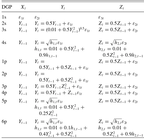
Table 1. Data-generating processes used in the simulations
(2008) test. The data-generating processes (DGPs) are detailed
inTable 1. The first four DGPs simulate data that allow to
illus-trate the size properties of the tests: DGP3s include the ARCH model of Engle (1982) and the DGP4s correspond to GARCH model of Bollerslev (1986). In the last six DGPs, the null hy-pothesis of conditional independence is not true and therefore serve to illustrate the power of the test: DGP1p–DGP3p exhibit linear and nonlinear Granger causality in the conditional mean and DGP4p–DGP6p correspond to nonlinear Granger causality through the conditional variance.
The BRT test depends on the bandwidthk, which is needed to estimate the copula densities. We takekequal to the integer part ofcT1/2forc=1,1.5,2. We consider various values of
kto evaluate the sensitivity with respect to the test results. This is common practice in nonparametric testing where no optimal bandwidth is available. In fact, this would typically involve an Edgeworth expansion of the asymptotic distribution of the test statistic, which is complex and left for future research. To keep the computing time in our simulation study reasonable, we consider the sample sizesT =200, 300 andB=200 bootstrap replications with resampling bandwidths chosen by the standard rule of thumb. We use 750 simulations to compute the empirical size and power. The computation time for the simulations is high because of the bootstrap replications within each Monte Carlo replication. For example, forc=2 it takes 27 days on a 2.67 GHz Dual Core processor to obtain the power results over the six DGPs.
To compare with our test, we also include the linear Granger noncausality test in the Monte Carlo experiment to appreciate the loss of power against nonlinear alternatives. This simply tests ifZt−1should enter the regression ofYt onYt−1.
Further-more, we compare with the conditional independence test of Su and White’s (2008), which is defined next. The latter test the null hypothesis on rescaled data by using densities instead of
copulas. First, consider the following fourth-order kernel func-tion k(u)=(3−u2)φ(u)/2, where φ(u) is the standard
nor-mal density. Then, if we choose the weighting functiona(w)=
d
partial derivative of a univariate density, h1 is a bandwidth
sequence, and Wt,i is the ith element of Wt =(Xt, Yt, Zt),
i=1,2, . . . , d. Following Gasser, M¨uller, and Mammitzsch (1985), it is assumed that 0≤v≤p−2, wherev=0 or 2 and
p is even. The choice of the kernel, k(v)(v=0,2), is crucial
to estimate the second-order partial derivatives. With respect to the bandwidth in the simulations, we take h=cn−1/8.5 for c=1,1.5,2.
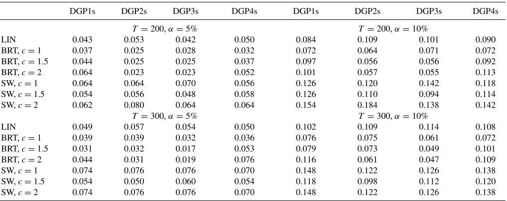
The size properties of our test, Su and White’s (2008)’s test, and linear Granger noncausality test are given in
Table 2. The linear test, say LIN, behaves well as expected
since the null hypothesis of conditional independence is satisfied. The BRT test tends to be slightly conservative for some DGPs. For example, for DGP2s with sample size 200 and c=1, the sizes are 2.5% instead of 5% and 6.4% instead of 10%. As expected, we also see that the realized size varies with the bandwidth k, in some cases the relation is positive and in others is negative. Further, it seems that Su and White’s (2008) test is oversized and this is the case for almost all DGPs and for 5% and 10% significance levels. Surprisingly, it seems that for several DGPs their size increases with the sample sizes we consider.
Table 2. Size properties of our test, Su and White’s (2008) test, and linear test
DGP1s DGP2s DGP3s DGP4s DGP1s DGP2s DGP3s DGP4s
T =200,α=5% T =200,α=10%
LIN 0.043 0.053 0.042 0.050 0.084 0.109 0.101 0.090
BRT,c=1 0.037 0.025 0.028 0.032 0.072 0.064 0.071 0.072
BRT,c=1.5 0.044 0.025 0.025 0.037 0.097 0.056 0.056 0.092
BRT,c=2 0.064 0.023 0.023 0.052 0.101 0.057 0.055 0.113
SW,c=1 0.064 0.064 0.070 0.056 0.126 0.120 0.142 0.118
SW,c=1.5 0.054 0.056 0.048 0.058 0.126 0.110 0.094 0.114
SW,c=2 0.062 0.080 0.064 0.064 0.154 0.184 0.138 0.142
T =300,α=5% T =300,α=10%
LIN 0.049 0.057 0.054 0.050 0.102 0.109 0.114 0.108
BRT,c=1 0.039 0.039 0.032 0.036 0.076 0.075 0.061 0.072
BRT,c=1.5 0.031 0.032 0.017 0.053 0.079 0.073 0.049 0.101
BRT,c=2 0.044 0.031 0.019 0.076 0.116 0.061 0.047 0.109
SW,c=1 0.074 0.076 0.076 0.070 0.148 0.122 0.126 0.138
SW,c=1.5 0.054 0.050 0.060 0.054 0.118 0.098 0.112 0.120
SW,c=2 0.074 0.076 0.076 0.070 0.148 0.122 0.126 0.138
Empirical size for a test at theαlevel based on 750 replications. The number of bootstrap resamples is B=200. LIN means linear test, BRT is our test, and SW means Su and White’s (2008) test. The bandwidthkis the integer part ofcT1/2.
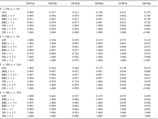
The power properties of our test, Su and White’s (2008) test, and linear Granger noncausality test are presented inTable 3. We observe that the linear test has only good power to detect linear Granger causality. In fact, the power is 1 for DGP1p. For the other DGPs that involve nonlinear dependence, the linear test fails to achieve considerable power. The BRT test has high power for all DGPs and the rise in its power from sample size 200 to 300 is important. Note also that generally the power of the BRT test goes down withc, which is not surprising since the bandwidth k in the BRT test plays the inverse role of a kernel bandwidth in nonparametric density estimation. Further, we see that the power of our test and Su and White’s (2008) test are more or less similar. But, of course, it is difficult to compare since Su and White’s (2008) test seems to have some size problem for the DGP’s and sample sizes under study.
5. EMPIRICAL APPLICATIONS
In this section, we consider two empirical applications to il-lustrate the importance of testing for nonlinear Granger causality and the usefulness of our nonparametric test in this context. In the first application, we use high-frequency equity index data to analyze the main explanations of the asymmetric volatility phe-nomenon and in the second application we examine the Granger causality between stock index returns and trading volume.
5.1 Application 1: Nonlinear Volatility Feedback Effect
One of the many stylized facts about equity returns is an asymmetric relationship between returns and volatility (here-after asymmetric volatility): volatility tends to rise following negative returns and fall following positive returns. The liter-ature has two explanations for the asymmetric volatility. The first one is the leverage effect and means that a decrease in the price of an asset increases financial leverage and the probabil-ity of bankruptcy, making the asset riskier, hence an increase
in volatility (see Black 1976; Christie1982). The second ex-planation is the volatility feedback effect, which is related to the time-varying risk premium theory: if volatility is priced, an anticipated increase in volatility would raise the rate of return, requiring an immediate stock price decline in order to allow for higher future returns (see Pindyck1984; French and Stambaugh 1987; and Campbell and Hentschel1992; among others).
Empirically, studies focusing on the leverage hypothesis— see Christie (1982) and Schwert (1989)—conclude that it cannot completely account for changes in volatility. For the volatility feedback effect, there are conflicting empirical findings. French and Stambaugh (1987) and Campbell and Hentschel (1992) found a positive relation between volatility and expected returns, while Turner, Startz, and Nelson (1989), Glosten and Runkle (1993), and Nelson (1991) found the relation to be negative but statistically insignificant. Using high-frequency data, Du-four, Garcia, and Taamouti (2008) measured a strong dynamic leverage effect for the first three days, whereas the volatility feedback effect is found to be insignificant at all horizons (see also Bollerslev, Litvinova, and Tauchen2006).
5.1.1 Data Description. We consider tick-by-tick trans-action prices for the S&P 500 Index futures contracts traded on the Chicago Mercantile Exchange, over the period January 1988–December 2005 (4494 trading days). Following Huang and Tauchen (2005), we eliminate a few days where trading was thin and the market was only open for a shortened ses-sion. Due to the unusually high volatility at the opening of the market, we omit the first five minutes of each trading day (see Bollerslev, Litvinova, and Tauchen 2006). We compute the continuously compounded returns over each five-minute in-terval by taking the difference between the logarithm of the two tick prices immediately preceding each five-minute mark. Because volatility is latent, it is approximated by either re-alized volatility or bipower variation. Daily rere-alized volatil-ity is defined as the summation of the corresponding high-frequency intradaily squared returns RVt+1= hj=1r
2 (t+j ,),
where r2
(t+j ,) are the discretely sampled -period returns.
Table 3. Power properties of our test, Su and White’s (2008) test, and linear test
DGP1p DGP2p DGP3p DGP4p DGP5p DGP6p
T =200,α=5%
LIN 0.999 0.337 0.213 0.126 0.163 0.153
BRT,c=1 0.995 0.996 0.979 0.989 0.904 0.785
BRT,c=1.5 0.971 0.993 0.931 0.997 0.931 0.759
BRT,c=2 0.943 0.979 0.873 0.997 0.912 0.728
SW,c=1 0.898 0.934 0.598 1.000 0.994 0.866
SW,c=1.5 0.994 0.998 0.816 1.000 0.994 0.966
SW,c=2 1.000 1.000 0.888 1.000 1.000 0.996
T =300,α=5%
LIN 1.000 0.354 0.250 0.113 0.172 0.143
BRT,c=1 1.000 1.000 0.995 0.999 0.981 0.931
BRT,c=1.5 0.997 1.000 0.991 1.000 0.988 0.913
BRT,c=2 0.989 0.997 0.971 1.000 0.991 0.883
SW,c=1 0.978 0.996 0.726 1.000 1.000 0.974
SW,c=1.5 1.000 1.000 0.926 1.000 1.000 0.998
SW,c=2 1.000 1.000 0.970 1.000 1.000 1.000
T =200,α=10%
LIN 1.000 0.436 0.284 0.175 0.239 0.233
BRT,c=1 0.995 0.997 0.932 0.991 0.939 0.869
BRT,c=1.5 0.987 0.996 0.957 0.997 0.967 0.841
BRT,c=2 0.968 0.992 0.923 0.997 0.948 0.833
SW,c=1 0.950 0.970 0.718 1.000 0.998 0.930
SW,c=1.5 0.998 1.000 0.878 1.000 0.994 0.986
SW,c=2 1.000 1.000 0.950 1.000 1.000 0.998
T =300,α=10%
LIN 1.000 0.442 0.327 0.176 0.253 0.209
BRT,c=1 1.000 1.000 0.996 0.999 0.988 0.944
BRT,c=1.5 0.999 1.000 0.996 1.000 0.995 0.948
BRT,c=2 0.992 0.999 0.984 1.000 0.996 0.935
SW,c=1 0.990 0.998 0.846 1.000 1.000 0.992
SW,c=1.5 1.000 1.000 0.954 1.000 1.000 1.000
SW,c=2 1.000 1.000 0.986 1.000 1.000 1.000
Empirical power for a test at theαlevel based on 750 replications. The number of bootstrap resamples is B=200. LIN means linear test, BRT is our test, and SW means Su and White’s (2008) test. The bandwidthkis the integer part ofcT1/2.
Properties of realized volatility were provided by Andersen, Bollerslev, and Diebold (2003) [see also Andersen and Boller-slev (1998); Andersen, et al. (2001); Barndorff-Nielsen and Shephard (2002a); Barndorff-Nielsen and Shephard (2002b) and Comte and Renault (1998)]. The bipower variation is given by sum of cross product of the absolute value of intradaily returns BVt+1= π2 hj=2|r(t+j ,)||r(t+(j−1),) |. Its
prop-erties are provided by Barndorff-Nielsen and Shephard (2003) (see also Barndorff-Nielsen, et al.2005).
5.1.2 Granger Causality Tests. To test for linear Granger causality, we estimate a first-order vector autoregressive model (VAR(1)). This yields the following results (t-statistics are be-tween brackets):
ˆ rt
ln(RVt)
=
0.001473[0.982]
−2.342446[−24.670]
+
−0.043375[−2.8974] 0.000150[0.995]
−6.000874[−6.3418] 0.764097[80.178]
×
rt−1
ln(RVt−1)
R2
=0.002
R2=0.597. (7) The results of linear Granger causality tests between daily return (r) and volatility (approximated by ln (RV)) are presented in (7) (see also Table 4). We find convincing evidence that return causes volatility. However, given thep-value of 0.320,we find that there is no impact (linear Granger causality) from volatility to return. Consequently, we conclude that there is a leverage effect but not a volatility feedback effect. Considering different orders for the above vector autoregressive model leads to the same conclusion. Further, replacing realized volatility (ln(RVt))
with bipower variation (ln(BVt)) also yields similar results.
To test for the presence of nonlinear volatility feedback and leverage effects, we consider the following null hy-potheses: H0:f(rt |rt−1, ln(RVt−1))=f(rt|rt−1) and H0:
f(ln(RVt)|ln(RVt−1), rt−1)=f(ln(RVt)|ln(RVt−1)),
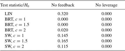
respec-tively. The results are presented inTable 4.
At a 5% significance level, we reject the Granger noncausality hypothesis for all directions of causality (from returns to volatil-ity and from volatilvolatil-ity to returns) and all values ofc. Contrary to
Table 4. P-values for linear and nonlinear Granger causality tests
Test statistic/H0 No feedback No leverage
LIN 0.320 0.000
BRT,c=1 0.000 0.000
BRT,c=1.5 0.000 0.000
BRT,c=2 0.020 0.000
SW,c=1 0.145 0.000
SW,c=1.5 0.165 0.000
SW,c=2 0.115 0.000
Linear and nonlinear Granger causality tests between returns (r) and volatility (approxi-mated by ln(RV)). LIN, BRT, and SW correspond to linear test, our nonparametric test, and Su and White’s (2008) test, respectively.
the linear Granger causality tests, we now confirm that both non-linear leverage and volatility feedback effects can explain the asymmetric relationship between returns and volatility. Consid-ering two lags for returns and volatility [rt−1, rt−2,ln(RVt−1),
ln(RVt−2)] in the previous null hypotheses, which corresponds
tod =5,leads to the same conclusion (thep-values are equal to zero) and confirms one more time the presence of nonlin-ear leverage and volatility feedback effects. As a comparison, we also implement Su and White’s (2008) test with the same weighting function as used in the simulations. As before, we find evidence in favor of the leverage effect, but their test does not seem able to pick up the volatility feedback effect.
5.2 Application 2: Granger Causality between Returns and Volume
The relationship between returns and volume has been subject to extensive theoretical and empirical research. Morgan (1976), Epps and Epps (1976), Westerfield (1977), Rogalski (1978), and Karpoff (1987) used daily or monthly data find a positive correlation between volume and returns (absolute returns). Gal-lant, Rossi, and Tauchen (1992)—considering a semiparametric model for conditional joint density of market price changes and volume—concluded that large price movements are followed by high volume. Hiemstra and Jones (1994) used a nonlinear Granger causality test proposed by Baek and Brock (1992) to ex-amine the nonlinear causal relation between volume and return and found that there is a positive bidirectional relation between them. However, Baek and Brock’s (1992) test assumes that the data for each individual variable is iid. More recently, Gervais, Kaniel, and Mingelgrin (2001) showed that periods of extremely high volume tend to be followed by positive excess returns, whereas periods of extremely low volume tend to be followed by negative excess returns. Gabaix et al. (2003) provided a theo-retical argument of square-root relationship between the trading volume and returns and argued that this relationship plays a key role in explaining the heavy-tailed phenomenon observer in financial returns. It is not easy to capture this square-root relationship using conventional tests based on linear parametric models; however, our nonparametric test will be able to detect it, since to apply the test the specification of functional form is not required. In this application, we reexamine the relationship between returns and volume using daily data on S&P 500 Index and its volume.
5.2.1 Data Description. The dataset comes from Yahoo Finance and consists of daily observations on the S&P 500 In-dex and its volume. The sample runs from January 1997 to January 2009 for a total of 3032 observations. We compute the continuously compounded changes in prices (returns) and trad-ing volume (volume growth rate) and we perform Augmented Dickey-Fuller tests (hereafter ADF-tests) for nonstationarity of the logarithmic price and volume and their first differences. Us-ing an ADF-test with only an intercept, the results show that all variables in logarithmic form are nonstationary. Using ADF-tests with both intercept and trend leads to the same conclusions. Based on the above stationarity tests, we model the first differ-ence of logarithmic price and volume rather than their level. Consequently, the causality relations have to be interpreted in terms of the growth rates.
5.2.2 Granger Causality Tests. To test for linear Granger causality between returns and volume, we estimate a first-order vector autoregressive model. This yields the following results (t-statistics are between brackets):
ˆ rt
ln(Vt)
=
4.96 10−5[0.20655]
0.001261[0.38206]
+
−0.068044[−3.75188] 0.000503[0.40386]
−1.338504[−5.36570] −0.323437[−18.8823]
×
rt−1
ln(Vt−1)
R2
=0.0047 R2
=0.1120. (8)
Equation (8) shows that the Granger causality from returns to volume is statistically significant at 5% significance level with
t-statistic equal to−5.366 (forp-values, seeTable 5). However, the feedback effect from volume to returns is statistically in-significant at the same significance level witht-statistic equal to 0.404.Considering different orders for vector autoregressive model leads to the same conclusion.
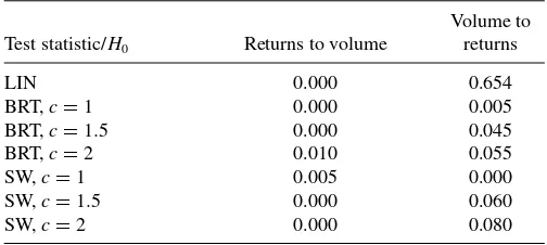
Since volume fails to have a linear impact on returns, next we examine the nonlinear relationships between the two variables using our nonparametric test and Su and White’s (2008) test. Thep-values are presented inTable 5. The latter shows that, at 5% significance level, our nonparametric test rejects clearly the null hypothesis of Granger noncausality from returns to volume, which is in line with the conclusion from the linear test. Further, our nonparametric test also detects a nonlinear feedback effect from volume to returns at the 10% significance level. Using Su and White’s (2008) test we find similar conclusions for testing Granger noncausality from both returns to volume and from volume to returns. Considering two lags for returns and volume growth rate [rt−1, rt−2, ln(Vt−1), ln(Vt−2)] in the previous
null hypotheses, which corresponds tod =5,leads to the same conclusion.
5.3 Discussion
Our approach has the advantage that it can test for Granger noncausality without imposing a model. Therefore, the rejection of noncausality in our empirical applications does not inform us about the exact nature of the causal relationship between the variables of interest and/or at which quantile level or moment
Table 5. P-values for linear and nonlinear Granger causality tests
Test statistic/H0 Returns to volume
Volume to returns
LIN 0.000 0.654
BRT,c=1 0.000 0.005
BRT,c=1.5 0.000 0.045
BRT,c=2 0.010 0.055
SW,c=1 0.005 0.000
SW,c=1.5 0.000 0.060
SW,c=2 0.000 0.080
Linear and nonlinear Granger causality tests between returns (r) and volume (ln(V)). LIN and BRT correspond to linear test and our nonparametric test, respectively.
of the distribution the causality exists. As shown in the above two applications, linear Granger causality tests are clearly not enough and might lead to wrong conclusions about the exis-tence or not of such a relationship. The statistical procedure proposed here can be viewed as pretest that allows us to see whether the variables are linked or not. Once we detect that there is a relationship, the next step is to identify the nature of the relationship or the level of the distribution where the two variables are connected. We give next three potential ways to pursue further analysis. First, the rejection of noncausality moti-vates the examination of the causality in higher-order moments. For example, Flannery and Protopapadakis (2002) reexamined the relationship between stock market returns and macroeco-nomic variables and argued that the effect of the latter variables on the former is possibly nonlinear. They provided convincing evidence of the impact of macroeconomic variables on the vari-ance of stock market returns. Second, we can consider quantile regression analysis. This will give a broader picture of the effect in various scenarios. For example, Lee and Yang (2006) showed the potential of improving quantile forecasting of output growth rate by incorporating information on money-income causality in quantiles, especially in the tails. Third, we can use neural networks to select the functional form that links the variables of interest. The latter approach is an interesting choice for flex-ible nonlinear modeling and is gaining attention in the area of stock-return prediction. For example, Qi (1999) considered neu-ral networks to model the nonlinear relationship between S&P 500 Index excess returns and financial and economic covariates.
6. CONCLUSION
A nonparametric copula-based test for conditional indepen-dence between two vector processes conditional on another one is proposed. The test statistic requires the estimation of the cop-ula density functions. We consider a nonparametric estimator of the copula density based on Bernstein polynomials. The Bern-stein copula estimator is always nonnegative and does not suffer from boundary bias problem. Further, the proposed test is easy to implement because it does not involve a weighting function in the test statistic, and it can be applied in general settings since there is no restriction on the dimension of the data. To ap-ply our test, only a bandwidth is needed for the nonparametric copula. We show that the test statistic is asymptotically pivotal under the null hypothesis, we establish local power properties, and we motivate the validity of the bootstrap technique that we
use in finite sample settings. A simulation study illustrates the size and power properties of the test. For the smallest sample size, our test has a somewhat lower size than the nominal level making our test conservative. This is in contrast with the test of Su and White’s (2008) that seems to overestimate the level. We consider two empirical applications to illustrate the usefulness of our nonparametric test. In these applications, we examine the Granger noncausality between different financial variables. Contrary to the general findings in the literature, we provide ev-idence on two alternative mechanisms of nonlinear interaction between returns and volatilities: the nonlinear leverage effect and the nonlinear volatility feedback effect.
There are several potential extensions of this article. First, an-alyze deeper the bandwidth selection for our nonparametric test, similar to the approach of Gao and Gijbels (2008) who tested the equality between an unknown and a parametric mean function. While respecting the size, their bandwidth maximizes the power of the test. In this respect, least squares cross-validation, similar to Li, Maasoumi, and Racine (2009), also deserves more atten-tion. Second, investigate analytically the small-sample proper-ties of our test along the lines of Fan and Linton (2003). Third, study the properties of our test under distance measures other than the Hellinger distance.
AKNOWLEDGMENTS
We thank Luc Bauwens, Christian Hafner, Todd Clark, Miguel Delgado, Jean-Marie Dufour, Jes´us Gonzalo, Oliver Linton, Jean-Francois Richard, Roch Roy, Carlos Velasco, two anonymous referees, an Associate Editor, and the Editor Jonathan Wright for several very useful comments. We also thank the participants of the 2008 Canadian Econometric Study Group, 7th World Congress in Probability and Statistics, Joint Meeting of the Statistical Society of Canada and the Societe Francaise de Statistique, 2009 UC3M-LSE Workshop, and sem-inar participants in Lille3, KUL, Maastricht University, UCL, University of Pittsburgh, the Federal Reserve Bank of Kansas City, and Humboldt University of Berlin for excellent comments that improved this paper. Financial support from the Spanish Ministry of Education through grants SEJ 2007-63098 is also acknowledged.
[Received June 2010. Revised October 2011.]
REFERENCES
Andersen, T., and Bollerslev, T. (1998), “Answering the Skeptics: Yes, Standard Volatility Models Do Provide Accurate Forecasts,”International Economic Review, 39, 885–905. [283]
Andersen, T., Bollerslev, T., Diebold, F., and Labys, P. (2001), “The Distribution of Realized Exchange Rate Volatility,”Journal of the American Statistical Association, 96, 42–55. [283]
Andersen, T. G., Bollerslev, T., and Diebold, F. X. (2003), “Parametric and Non-Parametric Volatility Measurement,” inHandbook of Financial Economet-ricsVol. 1, eds. Y. Ait-Sahalia and L. P. Hansen, Amsterdam: Elsevier-North Holland, pp. 67–138. [282]
Baek, E., and Brock, W. (1992), “A General Test for Non-Linear Granger Causality: Bivariate Model, Document de Travail”, Madison, WI, Iowa State University and University of Wisconsin. [276,284]
Barndorff-Nielsen, O., Graversen, S., Jacod, J., Podolskij, M., and Shephard, N. (2005), “A Central Limit Theorem for Realized Power and Bipower Vari-ations of Continuous Semimartingales,” Nuffield College working paper, Oxford University; forthcoming in Yu Kabanov and Robert Liptser (eds.),
From Stochastic Analysis to Mathematical Finance,Festschrift for Albert Shiryaev. New York: Springer-Verlag. [283]
Barndorff-Nielsen, O., and Shephard, N. (2002a), “Econometric Analysis of Realized Volatility and Its Use in Estimating Stochastic Volatility Models,” Journal of the Royal Statistical Society,Series B, 64, 253–280. [283] ——— (2002b), “Estimating Quadratic Variation Using Realized Variance,”
Journal of Applied Econometrics, 17, 457–478. [283]
——— (2003), “Power and Bipower Variation with Stochastic and Jumps”. Manuscript, Oxford: Oxford University Press. [283]
Beran, R. (1977), “Minimum Hellinger Distance Estimates for Parametric Mod-els,”The Annals of Statistics, 5, 445–463. [278]
Black, F. (1976), “Studies of Stock Price Volatility Changes,”Proceedings of the 1976 Meetings of the American Statistical Association, Business and Economic Statistics, pp. 177–181. [282]
Bollerslev, T. (1986), “Generalized Autoregressive Conditional Heteroskedas-ticity,”Journal of Econometrics, 31, 307–327. [281]
Bollerslev, T., Litvinova, J., and Tauchen, G. (2006), “Leverage and Volatility Feedback Effects in High-Frequency Data,”Journal of Financial Econo-metrics, 4(3), 353–384. [282]
Bouezmarni, T., Rombouts, J., and Taamouti, A. (2009), “Asymptotic Properties of the Bernstein Density Copula Estimator for Alpha Mixing Data,”Journal of Multivariate Analysis, 101, 1–10. [276,278,279]
Brock, W., Dechert, W., Scheinkman, J., and LeBaron, B. (1996), “A Test for Independence Based on the Correlation Dimension,”Econometric Reviews, 15, 197–235. [279]
Campbell, J., and Hentschel, L. (1992), “No News is Good News: An Asym-metric Model of Changing Volatility in Stock Returns,”Journal of Financial Economics, 31, 281–331. [282]
Carrasco, M., and Chen, X. (2002), “Mixing and Moment Properties of Various GARCH and Stochastic Volatility Models,”Econometric Theory, 18, 17–39. [279]
Chalak, K., and White, H. (2008), “Independence and Conditional Independence in Causal Systems,” Document de Travail, San Diego, CA, University of California. [275]
Chen, X., and Fan, Y. (2006a), “Estimation and Model Selection of Semipara-metric Copula-Based Multivariate Dynamic Models under Copula Misspec-ification,”Journal of Econometrics, 135, 125–154. [276]
——— (2006b), “Estimation of Copula-Based Semiparametric Time Series Models,”Journal of Econometrics, 130, 307–335. [276]
Chen, S. X., and Huang, T. (2007), “Nonparametric Estimation of Copula Func-tions for Dependent Modeling,”Canadian Journal of Statistics, 35, 265–282. [278]
Chen, X., Wu, W., and Yi, Y. (2009), “Efficient Estimation of Copula-Based Semiparametric Markov Models,”The Annals of Statistics, 37, 214– 4253. [276]
Christie, A. (1982), “The Stochastic Behavior of Common Stock Variances Value, Leverage and Interest Rate Effects,”Journal of Financial Economics, 3, 145–166. [282]
Comte, F., and Renault, E. (1998), “Long Memory in Continuous Time Stochas-tic Volatility Models,”Mathematical Finance, 8, 291–323. [283]
Deheuvels, P. (1979), La Fonction de D´ependance Empirique and Ses Propri´et´es: Un Test Nonparam´etrique D’ind´ependance, Bullettin de l’acad´emie Royal de Belgique, Classe des Sciences, pp. 274–292. [278]
Delgado, M. A., and Gonz´alez Manteiga, W. (2001), “Significance Testing in Nonparametric Regression Based on the Bootstrap,”The Annals of Statistics, 29, 1469–1507. [276,276]
Doukhan, P. (1994),Mixing: Properties and Examples, New York: Springer-Verlag. [279]
Doukhan, P., Fermanian, J.-D., and Lang, G. (2009), “An Empirical Central Limit Theorem with Applications to Copulas under Weak Dependence,” Statistical Inference for Stochastic Processes, 12, 65–87. [278]
Dufour, J.-M., Garcia, R., and Taamouti, A. (2008), “Measuring Causality be-tween Volatility and Returns with High-Frequency Data,” Document de Travail, Montreal, Universit´e de Montr´eal, and Madrid, Universidad Carlos III de Madrid. [282]
Dufour, J.-M., and Renault, E. (1998), “Short-Run and Long-Run Causality in Time Series: Theory,”Econometrica, 66, 1099–1125. [275]
Dufour, J.-M., and Taamouti, A. (2010), “Short and Long Run Causality Measures: Theory and Inference,” Journal of Econometrics, 154, 42– 58. [275]
Engle, R. (1982), “Autoregressive Conditional Heteroscedasticity with Esti-mates of the Variance of United Kingdom Inflation,”Econometrica, 50, 987–1007. [281]
Epps, T. W., and Epps, M. (1976), “The Stochastic Dependence of Security Price Changes and Transaction Volumes: Implication for the Mixture-of-Distributions Hypothesis,”Econometrica, 44, 305–322. [284]
Fan, J., and Yao, Q. (2003),Nonlinear Time Series: Nonparametric and Para-metric Methods, New York: Springer. [279]
Fan, Y., and Li, Q. (1996), “Consistent Model Specification Tests: Omitted Variables and Semiparametric Functional Forms,”Econometrica, 64, 865– 890. [276,276,278]
——— (1999), “Central Limit Theorem for Degenerate U-Statistics of Abso-lutely Regular Processes with Applications to Model Specification Tests,” Journal of Nonparametric Statistics, 10, 245–271. [279]
——— (2000), “Consistent Model Specification Tests: Kernel-Based Tests Ver-sus Bierens ICM Tests,”Econometric Theory, 16, 1016–1041. [276] Fan, Y., and Linton, O. (2003), “Some Higher-Order Theory for a Consistent
Non-Parametric Model Specification Test,”Journal of Statistical Planning and Inference, 109, 125–154. [285]
Fermanian, J., Radulovic, D., and Wegkamp, M. (2004), “Weak Convergence of Empirical Copula Processes,”Bernouilli, 10, 847–860. [278]
Fermanian, J., and Scaillet, O. (2003), “Nonparametric Estimation of Copulas for Time Series,”Journal of Risk, 5, 25–54. [278]
Flannery, M., and Protopapadakis, A. (2002), “Macroeconomic Factors Do Influence Aggregate Stock Returns,”Review of Financial Studies, 15, 751– 782. [285]
Florens, J., and Mouchart, M. (1982), “A Note on Non-Causality,” Economet-rica, 50, 583–591. [275]
Florens, J.-P., and Foug´ere, D. (1996), “Non-Causality in Continuous Time,” Econometrica, 64, 1195–1212. [275]
French, K. R., Schwert, G. W., and Stambaugh, R. (1987), “Expected Stock Returns and Volatility,”Journal of Financial Economics, 19, 3–30. [282] Gabaix, X., Gopikrishnan, P., Plerou, V., and Stanley, H. (2003), “A Theory of
Power-Law Distributions in Financial Market Fluctuations,”Nature, 423, 267–270. [284]
Gallant, R., Rossi, P., and Tauchen, G. (1992), “Stock Prices and Volume,” Review of Financial Studies, 5, 199–242. [284]
Gao, J., and Gijbels, I. (2008), “Bandwidth Selection in Nonparametric Kernel Testing,”Journal of the American Statistical Association, 103, 1584–1594. [285]
Gasser, T., M¨uller, H., and Mammitzsch, V. (1985), “Kernels for Nonparametric Curve Estimation,”Journal of the Royal Statistical Society,Series B, 47, 238–252. [281]
Gervais, S., Kaniel, R., and Mingelgrin, D. (2001), “The High-Volume Return Premium,”Journal of Finance, 56(3), 877–919. [284]
Gijbels, I., and Mielniczuk, J. (1990), “Estimating the Density of a Copula Function,”Communications in Statistics, 19, 445–464. [278]
Glosten, L. R., Jagannathan, R., and Runkle, D. E. (1993), “On the Relation Between the Expected Value and the Volatility of the Nominal Excess Return on Stocks,”Journal of Finance, 48, 1779–1801. [282]
Gouri´eroux, C., and Tenreiro, C. (2001), “Local Power Properties of Kernel Based Goodness of Fit Tests,”Journal of Multivariate Analysis, 78, 161– 190. [280]
Granger, C. W.J. (1969), “Investigating Causal Relations by Econometric Mod-els and Cross- Spectral Methods,”Econometrica, 37, 424–459. [275] Hiemstra, C., and Jones, J. (1994), “Testing for Linear and Nonlinear Granger
Causality in the Stock Price-Volume Relation,”Journal of Finance, 49(5), 1639–1664. [284]
Horowitz, J., and Spokoiny, V. (2001), “Adaptive, Rate-Optimal Test of a Parametric Mean-Regression Model Against a Nonparametric Alternative,” Econometrica, 69, 599–631. [280]
Huang, X., and Tauchen, G. (2005), “The Relative Contribution of Jumps to Total Price Variance,”Journal of Financial Econometrics, 3(4), 456–499. [282]
Karpoff, J. M. (1987), “The Relation between Price Changes and Trading Vol-ume: A Survey,”Journal of Financial and Quantitative Analysis, 22(1), 109–126. [284]
Kitamura, Y. (2001), “Asymptotic Optimality of Empirical Likelihood for Test-ing Moment Restrictions,”Econometrica, 69, 1661–1672. [276]
Lee, S., and Whang, Y.-J. (2009), “Nonparametric Tests of Conditional Treat-ment Effects,” DocuTreat-ment de Travail, London, University College London, and Seoul, Seoul National University. [276]
Lee, T., and Yang, W. (2006), “Money-Income Granger-Causality in Quantiles, Document de Travail,” Riverside, CA, University of California. [285] Li, Q., Maasoumi, E., and Racine, J. (2009), “A Nonparametric Test for Equality
of Distributions with Mixed Categorical and Continuous Data,”Journal of Econometrics, 148, 186–200. [285]
Linton, O., and Gozalo, P. (1997), “Conditional Independence Restrictions: Testing and Estimation,” Cowles Foundation Discussion Paper 1140, New Haven, CT, Cowles Foundation for Research in Economics, Yale University. [276]
Meitz, M., and Saikkonen, P. (2008), “Ergodicity, Mixing, and Existence of Moments of a Class of Markov Models with Applications to GARCH and ACD Models,”Econometric Theory, 24, 1291–1320. [279]
Morgan, I. (1976), “Stock Prices and Heteroskedasticity,”Journal of Business, 49, 496–508. [284]