Full Terms & Conditions of access and use can be found at
http://www.tandfonline.com/action/journalInformation?journalCode=ubes20
Download by: [Universitas Maritim Raja Ali Haji] Date: 12 January 2016, At: 23:13
Journal of Business & Economic Statistics
ISSN: 0735-0015 (Print) 1537-2707 (Online) Journal homepage: http://www.tandfonline.com/loi/ubes20
Inference in Panel Cointegration Models With Long
Panels
Rolf Larsson & Johan Lyhagen
To cite this article: Rolf Larsson & Johan Lyhagen (2007) Inference in Panel Cointegration
Models With Long Panels, Journal of Business & Economic Statistics, 25:4, 473-483, DOI: 10.1198/073500106000000549
To link to this article: http://dx.doi.org/10.1198/073500106000000549
Published online: 01 Jan 2012.
Submit your article to this journal
Article views: 96
Inference in Panel Cointegration Models
With Long Panels
Rolf LARSSON
and Johan LYHAGEN
Department of Information Science, Division of Statistics, Uppsala University, Uppsala, Sweden (Rolf.Larsson@dis.uu.se;Johan.Lyhagen@dis.uu.se)
This article presents a general likelihood-based framework for inference in panel vector autoregressive (VAR) models with cointegration restrictions. The cointegrating relationships are restricted to each cross section while the rest of the model is unrestricted. The homogeneous restriction of common cointegrating space is also considered. Asymptotic distributions of parameter estimators and the test statistics for the cointegrating rank and the homogeneous restriction are derived. The asymptotic distribution for the coin-tegrating rank is shown to be the convolution of the standard distribution of the trace statistic and theχ2
distribution. The homogeneous restriction test statistic is asymptoticallyχ2. A Monte Carlo simulation investigates the small-sample properties of the two tests. The empirical size of the test for the cointegrat-ing rank is well above the nominal. A Bartlett-corrected test statistic is shown to have size very close to the nominal. We give an empirical example for a consumption model, including consumption, income, and inflation as well as considering the monetary exchange rate model of Groen and Kleibergen.
KEY WORDS: Bartlett correction; Consumption; Panel data; Rank test.
1. INTRODUCTION
The seminal work of Engle and Granger (1987) on cointegra-tion has inspired an enormous amount of both theoretical and applied work. The reason for this is easy to understand, as the cointegrating vector can be interpreted as the long-run equilib-rium, which is of much interest to economists. From the simple one-equation Engle–Granger approach, the theoretical direc-tion has been in the multivariate setting proposed by Johansen (1988) and then toward generalizations such as seasonal coin-tegration (see Lee 1992; Johansen and Schaumburg 1998) and cointegration forI(2)processes (see Johansen 1997). From an economic point of view, there has been an interest in involv-ing more than one country in the analysis, as it is reasonable to assume that an economic theory should hold for more than one country. In fact, economic theories should be valid for all countries as long as they are not fundamentally different. Of course, this does not imply that all parameters are equal—a re-striction that can be tested for—but that the statistical model should be reasonably similar and the statistical properties of economic variables should be the same across countries. This has inspired the work toward panel unit roots and panel coin-tegration, successfully applied on, for example, the purchasing power parity for exchange rates; see Papell (1997), O’Connell (1998), and Jacobson, Larsson, Lyhagen, and Nessen (2002).
Statistically, a panel approach has the advantage of increas-ing the degrees of freedom with the consequence of better size and power properties of statistical tests. Unfortunately, the panel approach also increases the risk of misspecifying the model, which worsens the size properties. Hence, it is impor-tant to have a rich variety of models to choose from and well-developed testing procedures to distinguish between them.
Compared to most previous work on panels and unit roots/co-integration (see, e.g., Levin, Lin, and Chu 2002; Im, Pesaran, and Shin 2003), this article focuses on multivariate cointegra-tion and extends the previous work by Larsson, Lyhagen, and Löthgren (2001) and Groen and Kleibergen (2003) where the former assumes completely independent cross sections and the latter dependency only through contemporary disturbances. [As
a referee pointed out, our model may be viewed as a restricted version of a quite large vector error correction model (VECM) model of the type suggested by Boswijk 1995.] However, our simulations show that ignoring cross-sectional dependencies will severely distort the test performed. The block-diagonality restriction of the adjustment parameters in Groen and Kleiber-gen (2003) is relaxed, yielding a more flexible model. The re-laxation of the block-diagonal structure is appealing from an economic perspective. Often the economic theory used is ap-plied on a country-by-country basis. Hence, it is plausible that the cointegrating vectors operate country by country; that is, the assumption of block-diagonal cointegrating vectors seems real-istic. An unrestricted adjustment matrix implies that the equi-librium error of one country helps the other countries to pull the process toward the equilibriums. For example, in the mon-etary exchange model of Groen and Kleibergen (2003), an ex-cess money supply in the U.K. will affect the equilibrium errors between the money supply, relative real income, and exchange rates for France and Germany. This behavior of the model is realistic as the capital market is very international.
The asymptotic distribution of the likelihood ratio test for the number of cointegrating relationships is derived. This dis-tribution may be described as the convolution of two indepen-dent variates: the first one following the well-known asymptotic distribution of the trace test (a Dickey–Fuller-type distribution) and the second one being asymptotically χ2. Furthermore, a likelihood ratio test of common cointegrating space is proposed, and it is shown that the asymptotic distribution isχ2. We also derive the asymptotic distribution of the likelihood ratio test of the null of a block-diagonal adjustment matrix, as in Groen and Kleibergen (2003), against the alternative of no restriction on the adjustment matrix. This isχ2as well.
A Monte Carlo simulation is performed to analyze the small-sample properties of the two tests. The test for common coin-tegrating space has sufficiently good size and power properties
© 2007 American Statistical Association Journal of Business & Economic Statistics October 2007, Vol. 25, No. 4 DOI 10.1198/073500106000000549 473
while the test for cointegrating rank does not. This result makes us propose the use of a Bartlett-corrected test statistic, which has the desired properties, that is, a size very close to the nomi-nal one.
Two empirical examples are carried out. The first example concerns two groups. The groups consist of countries that are, in some sense, similar. The first contains some larger economies (Japan, the U.K., and the United States), and the second group contains the major Nordic countries (Denmark, Finland, Nor-way, and Sweden). The variables are income, consumption, and inflation. The result is that both groups have one cointegrat-ing vector. The test of common cointegratcointegrat-ing space is rejected for both groups. The hypothesis of a block-diagonal adjust-ment matrix, given the model by Groen and Kleibergen (2003), is rejected against the alternative of a model with no restric-tion on the adjustment matrix. The second empirical example deals with the monetary exchange rate model of Groen and Kleibergen (2003). Here, we do not reject the null of a block-diagonal adjustment matrix.
The number of parameters in the model increases rapidly with the number of cross sections, which is why, as seen from the preceding empirical example, the number of cross sections used is rather small. This can be criticized from the traditional large panel view. We rather feel that this approach should be compared to the time series approach where one cross section at a time is analyzed. In that respect, important insights may be gained from treating more than one cross section simultane-ously, because, when studying the countries separately, cross-country dependence is completely overlooked.
For typical lengths of yearly macro time series, a cross-sectional dimension larger than 4 or 5 (say) would probably demand a statistical panel model with fewer parameters than ours; see, for example, Bai and Ng (2004).
The outline of this article is as follows. In the next section the general model and the two special cases are presented, and esti-mation is discussed in Section 3. Section 4 considers asymptotic results for the distribution of parameters and the likelihood ra-tio tests. To evaluate the small-sample properties a Monte Carlo simulation is carried out in Section 5, and the empirical exam-ples are presented in Section 6. A conclusion ends the article.
2. THE GENERAL MODEL
Consider a panel dataset that consists of a sample ofNcross sections (e.g., industries, regions, or countries) observed over T time periods. Leti=1, . . . ,Nindex the groups,t=1, . . . ,T the sample time period, andj=1, . . . ,pthe variables in each group. Then yijt denotes the ith group and thejth variable at
timet. The observedpvector for groupiat time periodtis given byy′it=(yi1t,yi2t, . . . ,yipt)′. Define Yt= [y′1t,y′2t, . . . ,y′Nt]′as theNpvector of the panel of observations available at timeton thepvariables for theNgroups.
The regression that is the basis for our work is ⎡
To continue, we impose some structure on this model. First, we consider a reduced rank specification of the panel model where the matrixis of rankNr, 0≤r≤p, specified as=
αcontains the short-run coefficients andβ the long-run coeffi-cients, whereβii≡βieach of rankr.
The block matrix elements of are given by ij = N
k=1αikβkj′ =αijβj′ due to the restriction thatβij=0 ∀i=j.
In a more compact notation, the model can be written as
Yt=μ+αβ′Yt−1+
m−1
k=1
ŴkYt−k+εt. (6)
This general model allows a simultaneous modeling of the long-run relationships between several variables for a panel of groups with heterogeneous long-run cointegration relationships within each group. Because of the restrictionβij=0 ∀i=j,
cointegrating relationships are only allowed within each of the N groups in the panel. These cointegrating relationships are
contained in the matrixβ′Yt−1, which consists of ther cointe-grating relationships for each individual,βi′yit−1,i=1, . . . ,N. However, the model allows for an important short-run depen-dence between the panel groups, because αij is not restricted
to 0 fori=j. More specifically, the off-diagonal elements in =αβ′, which are given byij=αijβj′fori=j, represent the
short-run dependencies of the changes in the series for groupi that are due to long-run equilibrium deviations in groupj. As in the standard single-group model, the diagonal element of, ii=αiiβi′, represents the short-run adjustments in groupi
re-sulting from a deviation from long-run equilibrium in groupi. Larsson et al. (2001) considered a similar heterogeneous panel data model under cointegration restrictions, with the added restriction that no dependencies are allowed between the panel groups. That is, the off-diagonal block elements of the matricesα,Ŵ, andare 0. With this additional restriction, the model is completely heterogeneous, and the panel groups are modeled individually as
yit=μi+αiβi′yit−1+
m−1
k=1
Ŵii,kyit−k+εit,
i=1, . . . ,N,t=1, . . . ,T. (7) Groen and Kleibergen (2003) relaxed the assumption of block diagonality of in this model. In other words, their framework is a special case of the one in this article with block-diagonalandŴkmatrices.
3. STATISTICAL ANALYSIS
3.1 Tests
Our first issue is to estimate the cointegrating rankr in the model (6). As in Johansen (1995b), we accomplish this by se-quentially testing
H(r): rank()≤Nr, (8) where=αβ′ withα andβ as in (4) and (5), respectively, against the alternative
H(p): rank()≤Np. (9) Observe that rank()is restricted to be a multiple ofN. More-over, if rank()=Np, the block diagonality of β is super-fluous. Under our restrictions on , it is easily realized that the consistency property of the sequential testing procedure of Johansen (1995b) also holds here.
Given the assumption of equal rank, the homogeneity hy-pothesis that the cointegrating vectors in the panel span the same space for each of the individual groups in the panel is nat-ural. That is, the second homogeneity hypothesis we consider is given by
H0:β1=β2= · · · =βN=β0 (10)
(observe thatβ0is arbitrary) against the alternative
H1:βi=βj for somei,j. (11)
Note that the homogeneous long-run coefficient β0 is not uniquely determined. Instead, the homogeneity hypothesis is the hypothesis that the long-run coefficientsβi span the same
space. This is seen because ifβ1=β2Rfor somer×rmatrixR of full rank, then we may writeαijβ1′=αij∗β2′ withα∗ij=αijR′,
whereαijis an arbitrary block ofαin (4).
Under the null hypothesis of homogeneity, the matrix of long-run coefficientsβ can be written asβ=IN⊗β0, and the general model is given by
Yt=μ+α(IN⊗β0′)Yt−1+
m−1
k=1
ŴkYt−k+εt. (12)
3.2 Estimation
In this section we discuss the estimation of the model in (6) with the two sets of restrictionsβ=diag(β1, . . . , βN)andβ=
IN⊗β0.
Observe that, for small enoughT, it may not be possible to estimate the parameters of the model. For example, if the lag lengthmis 1, the number of parameters is at mostN2p2. As we haveNpequations, each equation must haveNpobservations to give an exactly identified system. Because the right side con-sists of lagged left-side variables, one observation is lost, so the number of time units used must be at leastT=Np+2.
3.2.1 Individual Cointegrating Relationships. The re-strictionβ=diag(β1, . . . , βN)may be written asβ=(H1(p)β1, . . . ,H(Np)βN), whereHi(p)is anNp×p matrix of 0’s except in
theith block where it is a unit matrix, that is,
Hi(p)=[ 0 · · · 0 Ip 0 · · · 0 ]′. (13)
Estimation of such kinds of restrictions is discussed in, for example, Johansen (1995a, b). The estimation procedure is to estimate H1(p)β1 in a reduced rank regression, where
H2(p)β2, . . . ,HN(p)βN have been concentrated out. Continue by
estimating H2(p)β2 given H(1p)β1,H(3p)β3, . . . ,H(Np)βN. When
HN(p)βNhas been estimated, restart the estimation with the new
values of H(1p)β1, . . . ,H(Np)βN. Repeat until convergence. For
starting values, we propose using the βi found when doing a
standard cointegrating analysis for theith cross section. 3.2.2 Homogeneous Cointegrating Relationships. Esti-mating (6) using the method proposed by Johansen (1988), we get the unrestricted estimator of β, which, with probabil-ity 1, does not satisfy the restriction β=IN⊗β0. Hence, it cannot be used to estimate the model we are interested in. Instead, we propose using the switching method of Boswijk (1995). (This method was proposed in a more general setting by Hansen 2002.) It is possible to numerically maximize the likelihood, but this is probably more time consuming than the switching method when largeNandpare considered, although Boswijk (1995) discussed an example when Newton–Raphson will reach optimum in one step and the switching converges slowly to optimum. See also Johansen (1995a) for a discussion on optimization versus switching methods.
For ease of exposition, we consider the model in (12) without a constant (μ=0) and short-run dynamics, which is the same as assuming that these terms have been concentrated out. Pre-multiply with the inverse of the square root of the covariance matrix ofεt, that is, with−1/2, to get
−1/2Yt=−1/2α(IN⊗β0′)Yt−1+−1/2εt, (14)
or, equivalently,
Y˜t=α(IN⊗β0′)Yt−1+et, (15)
where we used the notationY˜tandαfor−1/2Ytand−1/2α,
respectively, and where E(ete′t)=Ip. Using the relationship
vec(ABC)=(C′⊗A)vec(B), we have
Y˜t=(Yt′−1⊗α)vec(IN⊗β0′)+et. (16)
Define the matrixHof sizeN2rp×rpas
H= ⎡ ⎢ ⎢ ⎢ ⎣
Ip⊗δN1 ⊗Ir
Ip⊗δN2 ⊗Ir
.. . Ip⊗δNN⊗Ir
⎤ ⎥ ⎥ ⎥
⎦, (17)
whereδNi is an N×1 vector of 0’s except for a 1 in the ith position. Then vec(IN⊗β0′)=Hvec(β0′). Note that the inverse
ofH′Hexists; that is, it isN−1Irp. Substitute this into (16):
Y˜t=(Yt′−1⊗α)Hvec(β ′
0)+et. (18)
The ordinary least squares (OLS) estimator of vec(β′)is then
((Yt′−1⊗α)H)′((Yt′−1⊗α)H)−1((Yt′−1⊗α)H)′Y˜t. (19)
This shows that, for a given value ofα and, we may esti-mateβ. The problem of estimatingαandfor given values of β is much simpler: Estimateαin (6) by regression ofYt
on β′Yt−1, corrected for (Yt−1, . . . , Yt−m+1). This regres-sion also gives an estimate of . The switching algorithm is that, for given initial values of β, estimateα and, then for these estimated values estimateβ. Repeat until the increase of the likelihood is sufficiently small. The mean of the estimated βifound when doing a standard cointegrating analysis for the
ith cross section is used as starting value forβ0.
4. ASYMPTOTIC DISTRIBUTIONS
In this section we give the asymptotic distribution of the likelihood ratio test for the cointegrating rank, that is, the test of H(r) against H(p) as given in (8) and (9), respec-tively. Then, given the rank, the model with the homogene-ity restriction β =IN⊗β0 is tested against the model with β=diag(β11, . . . , βNN). The proofs are given in the Appendix,
where we also state and prove a theorem about the asymptotic distribution of the maximum likelihood (ML) estimator ofβ.
First, we need some definitions. Define α⊥ as an Np× N(p−r) matrix (the choice of it is not unique) that fulfills the requirementsα⊥′ α=0,α′α⊥=0, and(α, α⊥)has full rank (Np), and similarly forβ⊥. Consequently, we may chooseβ⊥≡ diag(β1⊥, . . . , βN⊥). Furthermore, lettingŴ≡INp− mk=−11Ŵk,
we need the following assumption, for ruling out processes in-tegrated of order higher than 1 (cf. Johansen 1995b, p. 49).
Assumption A. The matrix α⊥′ Ŵβ⊥ has full rank. Further-more, the roots of the characteristic polynomial
A(z)=(1−z)INp−αβ′z− m−1
i=1
Ŵk(1−z)zi
are outside the complex unit circle or 1.
4.1 The Test for Cointegrating Rank
We are now ready to formulate our first main result. Observe that we requirer>0. Ifr=0, the block-diagonal structure has no meaning, and, in this case, the asymptotics is the same as in Johansen (1995b, chap. 6). Moreover, observe the short-hand notation of integrals, that is,FF′=01F(t)F(t)′dt.
Theorem 1. LetQTbe the maximum likelihood ratio test
sta-tistic for the test ofH(r)againstH(p). Under Assumption A, if r>0, we have that, asT→ ∞,
−2 logQT w
→U+V,
whereV isχ2withN(N−1)r(p−r)degrees of freedom, in-dependent ofU. The quantityUhas the form
U=tr
dB F′
FF′ −1
F dB′
.
Here, if μ=0, F=B is an N(p−r)-dimensional standard Wiener process (with mean 0 and covariance matrixIN(p−r)). If μ=0 andα⊥′ μ=0,Bis anN(p−r−1)-dimensional standard Wiener process with componentsBi andFis{N(p−r−1)+
1}-dimensional with components
Fi(u)≡
⎧ ⎪ ⎪ ⎨ ⎪ ⎪ ⎩
Bi(u)−
1
0
Bi(t)dt, i=1, . . . ,N(p−r−1)
u−1
2, i=N(p−r−1)+1. Ifμ=0 andα⊥μ=0,Bis anN(p−r)-dimensional standard Wiener process with componentsBiandFis{N(p−r)+1}
-di-mensional with components
Fi(u)≡
Bi(u), i=1, . . . ,N(p−r)
1, i=N(p−r)+1.
In other words, the limit distribution of our test for cointe-grating rank equals the convolution of a well-known Dickey– Fuller-type distribution (which arises as the asymptotic distri-bution for the corresponding rank test in a model without any restrictions onβ; cf. Johansen 1995b) and an independent χ2 variate. It is fairly easy to simulate this distribution in the usual fashion, approximating the Wiener process by a random walk. Moreover, considering the moments ofUas known (see, e.g., the simulation results of Doornik 1998), our representation pro-vides us with a simple way of calculating the asymptotic mo-ments of our test statistic. Note that proposition 3 in Groen and Kleibergen (2003) states a similar distribution, but in their case theχ2part arises due to a common cointegrating space restric-tion while here it is due to the block diagonality of the cointe-grating vectors.
The proof of the theorem builds on a decomposition of the test into two: the test of reduced rank in the full model (with no restriction onβ) and the test of the block-diagonality restric-tion onβ, given reduced rank. The former is studied in detail in, for example, Johansen (1995a), so what remains is to ana-lyze the block-diagonality test and to show that the two tests are independent of each other underH(r). The asymptotic distrib-ution of the block-diagonality test doesnotfollow as an imme-diate special case of, for example, theorem 13.10 in Johansen (1995b), because under block diagonality,β is not identified in the sense of that theorem unlessr=1. However, theorem C.1
of Johansen (1991), which deals with smooth hypotheses onβ, may be applied. From this theorem, it follows immediately that the asymptotic distribution isχ2, and it is not too difficult to find the number of degrees of freedom. Showing independence of the rank test requires some extra work; see the Appendix for further details.
We end this section by observing how our asymptotic dis-tribution differs from corresponding rank test disdis-tributions in related work. In Larsson et al. (2001), independence between individuals was assumed, andN was treated as a large quan-tity. Hence, their asymptotic distribution, asboth NandT tend to∞, is normal when correcting for the first two moments of the Dickey–Fuller distribution. Groen and Kleibergen imposed a mild dependence between individuals through the covariance matrix. This results in an asymptotic distribution, which is the same as what would be obtained in Larsson et al. (2001) by lettingT only tend to∞, that is, the distribution of a sum ofN independent Dickey–Fuller-distributed random variables.
4.2 Testing Homogeneous Cointegrating Relationships
Our next step is to find the asymptotic distribution of the log-likelihood ratio test, given the rank, of the homogeneity hypoth-esis
H0:β1=β2= · · · =βN=β0
against the alternative
H1:βi=βj for somei,j.
In view of earlier literature on similar restriction tests (see, e.g., Johansen 1995b), the result that this distribution isχ2, given in Theorem 2, should not come as a surprise to the reader. The number of degrees of freedom,(N−1)r(p−r), is natural be-cause, as is easily seen, this is the difference of the numbers of free parameters under the different hypotheses. Moreover, note that this result is identical to the corresponding result in Groen and Kleibergen (2003; prop. 3, reformulated as a test of com-mon cointegrating space, given the reduced rank).
Theorem 2. Under Assumption A, given the rank r>1, the log-likelihood ratio test statistic for test ofH0:β1= · · · = βN=β0 againstH1:βi=βjfor somei,jis, underH0 and as
T→ ∞, asymptotically χ2 distributed with (N−1)r(p−r) degrees of freedom.
4.3 Testing Block Diagonality of the Adjustment Matrix
As the model of Groen and Kleibergen (2003) is a special case of the model proposed here, it is possible to test their block-diagonality restriction of the adjustment matrix. This means that allαij of (4) with i=jare 0. The following
theo-rem gives the asymptotic distribution of this test.
Theorem 3. Under Assumption A, the log likelihood ra-tio test statistic for test of H∗
0:αij =0 for all i=j against
H1:αij=0 for somei=jis, underH∗0and asT→ ∞,
asymp-toticallyχ2distributed withN(N−1)prdegrees of freedom.
5. A SIMULATION STUDY
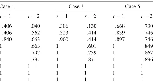
It is of practical interest to evaluate how well the asymp-totic distribution of the likelihood ratio test for the cointegrating rank mimics the small-sample distribution. To this end, a Monte Carlo simulation is a suitable tool to use. The length of the random walk approximating the Brownian motion is 800 and the number of replicates is 100,000. For the analysis of small-sample properties, the small-sample sizes we consider are T=100, 200, 500, and 1000. Because of time constraints, the number of replicates is limited to 10,000. The data-generating process is gained by estimating the models of interest on data. For simplic-ity, the variables are demeaned, and the models are estimated without deterministic components. The variables used are (log of) consumption, income, and inflation for Japan, the U.K., and the United States, that is,n=p=3; see the next section. The largest absolute values of the eigenvalues of the data-generating processes, referred to as case 1, case 3, and case 5, are shown in Table 1. All of them are relatively far from 1; hence, the processes for rank 1 and rank 2 are sufficiently separated.
The simulations are carried out in Gauss 3.2. Following are the different cases simulated for ranks 1 and 2 andm=1:
1. β=IN⊗β0withαandunrestricted. 2. As in case 1, but with block-diagonal.
3. β=diag(β11, . . . , βNN)withαandunrestricted.
4. As in case 3, but with bothαandblock diagonal. 5. As in case 4, but withm=2.
Cases 1, 3, and 5 are estimated from data. Case 2 is gained by restricting case 1, and case 4 is obtained by restricting case 5. Unfortunately, and contrary to the ordinary case, the conver-gence to the asymptotic distribution is slow; see Tables 2 and 3. This is especially true for case 5 wherem=2. This motivates the use some kind of small-sample method such as Bartlett cor-rection. Moreover, it seems that the size properties for the two different ranks considered are quite similar.
For the test of β =IN⊗β0 versus β=β =diag(β11, . . . , βNN), the size of the test is much better; see Tables 4 and 5.
Furthermore, the power is extremely good; the power is 1 even for the smallest sample size(T=100).
5.1 Bartlett Correction
The Bartlett correction was introduced by Bartlett (1937); see Cribaro-Neto and Cordeiro (1996) for a nice treatment of
Table 1. Absolute values of the eigenvalues of some data-generating processes used in the simulation study
Case 1 Case 3 Case 5
r=1 r=2 r=1 r=2 r=1 r=2
.406 .040 .306 .130 .668 .730
.406 .562 .323 .414 .839 .746
.840 .663 .900 .414 .897 .746
1 .663 1 .601 1 .849
1 .797 1 .759 1 .867
1 .797 1 .871 1 .896
1 1 1 1 1 1
1 1 1 1 1 1
1 1 1 1 1 1
NOTE: In case 5, only the largest eigenvalues are given in the table.
the subject. In cointegration analysis, it has been used by, for example, Jacobson and Larsson (1999) with only a small size improvement compared to using the asymptotic distribution. This is probably due to the good performance of the latter. In our case, where the size of the test is far away from the nomi-nal for sample sizes up toT=500, Bartlett correction may be useful. The articles of Johansen (2000, 2002) are also highly relevant. The former considers Bartlett correction of tests for restrictions on the cointegrating space (however, not the block-diagonal restriction treated in our article). The latter presents a small-sample correction of the test for cointegrating rank of Bartlett type.
To give a brief description of Bartlett correction, consider the statisticCT for sample sizeTand letC∞be its asymptotic counterpart andEthe expectation operator. Then, the Bartlett-corrected statistic is
CT∗=ECT
C∞ EC∞
.
Hence, ifx(aT)andxaare the 100a% fractiles of the distributions
ofCTandC∞, respectively, we have, approximatingCT byC∗T,
P(C∞>xa)=a=P
CT>x(aT)
≈PC∗T>x(aT)=P
C∞> EC∞
ECT
x(aT)
.
Consequently, we get the fractile approximation
x(aT)≈ ECT
EC∞ xa.
To get explicit formulas, Johansen (2000, 2002) expanded ECT/EC∞ inT−1and neglected high-order terms. This prac-tice has the drawback of producing an extra approximation er-ror. To avoid this problem, we follow the route of Jacobson and Larsson (1999) and simulateECT/EC∞. To simulateECT, we
first estimate the model under the null. Given the estimates, we generate new series and calculate the test statistic. Then, repeat-ing a large number of times (in our case, 10,000), we estimate ECT with the mean of the estimated test statistics.
The result is that the Bartlett-corrected statistic works ex-tremely well for all sample sizes and cases considered. The size is very close to the nominal 5%; see Table 6 for rank 1. The result for rank 2 is very similar and, hence, is not reported.
5.2 Comparison With Groen and Kleibergen
If a block-diagonal restriction is set on the adjustment para-meters, that is, on (4), then the model is the one proposed by Groen and Kleibergen (2003). Hence, it is of interest to com-pare the performance of the two competing models within a Monte Carlo framework. Case 4 is a correct data generating process (DGP) for their model, whereas case 3 is a misspecified one where the misspecification lies in the non–block diagonal-ity of the adjustment parameters. The results are displayed in Table 7. For case 4, the size is rather good for all samples. It is better than only using the asymptotic distribution of the more general model, but not as good as using the Bartlett-corrected one. The explanation for this is that estimating more parameters decreases the efficiency of the test, a well-known result. The size properties of the misspecified model are much worse and
Table 2. Size for small samples, 5% test, and rank=1
Case T=100 T=200 T=500 T=1,000
1 .293 .149 .089 .072
2 .295 .152 .089 .069
3 .314 .173 .091 .076
4 .251 .124 .077 .067
5 .846 .408 .156 .097
NOTE: The critical value is 97.20.
Table 3. Size for small samples, 5% test, and rank=2
Case T=100 T=200 T=500 T=1,000
1 .253 .135 .082 .063
2 .238 .126 .073 .063
3 .226 .124 .081 .068
4 .316 .151 .086 .070
5 .734 .343 .133 .086
NOTE: The critical value is 39.43.
Table 4. Size and power for small samples of test for common cointegrating space, four degrees of freedom, 5% test, and rank=1
Case T=100 T=200 T=500 T=1,000
1 .110 .049 .055 .051
2 .094 .073 .059 .054
3 1 1 1 1
4 1 1 1 1
5 1 1 1 1
Table 5. Size and power for small samples of test for common cointegrating space, 5% test, and rank=2
Case T=100 T=200 T=500 T=1,000
1 .120 .074 .055 .055
2 .104 .074 .059 .052
3 1 1 1 1
4 1 1 1 1
5 1 1 1 1
Table 6. Size for small samples, Bartlett-corrected test, and rank=1
Case T=100 T=200 T=500 T=1,000
1 .045 .049 .047 .050
2 .045 .048 .047 .048
3 .045 .048 .046 .049
4 .049 .050 .047 .051
5 .038 .047 .048 .049
NOTE: A 5% significance level is used.
Table 7. Sizes for the rank test by Groen and Kleibergen and for the block diagonality of adjustment parameters test
Rank Case T=100 T=200 T=500 T=1,000
1 3 .3376 .3223 .3272 .3404
1 4 .0868 .0677 .0580 .0544
2 3 .1576 .1494 .1450 .1500
2 4 .0786 .0635 .0573 .0556
1 4 .0958 .0691 .0568 .0564
2 4 .1905 .0979 .0635 .0581
NOTE: A 5% significance level is used. The critical value for the null of rank 1 is 77.50 and for rank 2 26.97. The block-diagonality test isχ2distributed with 18 and 36 degrees of freedom, respectively.
do not improve with increased sample size. The simulation re-sults indicate that the distribution is shifted as the size is rather constant over the sample size. This can also be expected as the test is the sum of the unrestricted cointegrating rank test pro-posed by Johansen (1988) and a (asymptotically independent) χ2test for the restrictions on the adjustment parameters.
A small Monte Carlo simulation was also performed to an-alyze the size properties of a test of block diagonality of the adjustment parameters. For the small sample sizes, the test is oversized but not extremely much. As could be expected, the case for rank 2 is worse than that for rank 1, because the rank 2 case involves more parameters. These results are shown in the last two rows of Table 7.
6. EMPIRICAL EXAMPLES
In this section we estimate a standard consumption function of the type considered by Davidson et al. (1978) for two ho-mogeneous groups of Organization for Economic Cooperation and Development (OECD) countries over the 35-year period 1960–1994. The two groups are (1) Japan, the U.K., and the United States; and (2) Denmark, Finland, Norway, and Swe-den. The data are obtained from the OECD CD–ROM Statis-tical Compendium, edition 02#1997. We consider the hetero-geneous panel error correction model with variable vector for each country given by
Yit=(cit,ydit, pit)′,
wherecit is the logarithm of real consumption per capita,yditis
the logarithm of real disposable income per capita, andpitis
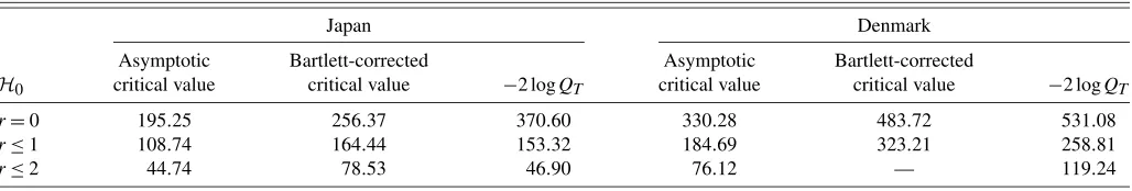
the rate of inflation. We follow Pesaran, Shin, and Smith (1999) in the definition of the variables: Consumption is measured by the logarithm of total private consumption per capita and infla-tion by the change in the logarithm of the consumpinfla-tion deflator, and national disposable income deflated by the consumption deflator is used as measure of income. Furthermore, a model with an unrestricted constant is used, and the number of lags ism=1 as the Schwarz criterion rejects a higher lag structure. The results of the likelihood ratio tests are given in Table 8. The Bartlett-corrected critical values are obtained by using the estimated model as a data-generating process when calculating the sample mean. A bootstrap approach like the one proposed by Gredenhoff and Jacobson (2001) could be used, but with the good size properties of the Bartlett critical values we do not think that a bootstrap is necessary.
For the group that consists of Japan, the U.K., and the United States, the estimated number of cointegrating vectors is 1 when using the Bartlett-corrected critical values, and the same is
true for the group that consists of Denmark, Finland, Nor-way, and Sweden. Note that if the asymptotic critical values were used, the estimated rank would be 3 for both groups. The Bartlett-corrected critical value for the Denmark group and rank 2 could not be calculated because the estimated model has roots larger than 1; hence, numerical (and theoretical) problems arose. The tests of common cointegrating space give test statis-tics of 31.38 and 31.01, respectively, and should be compared to χ.295,df=4=9.49 andχ.295,df=6=12.59. Hence, both groups re-ject the null of common cointegrating space. Testing the null of a block-diagonal adjustment matrix, as in Groen and Kleibergen (2003), the test statistics are 59.56 and 124.83 and should be compared toχ.295,df=18=28.87 andχ.295,df=36=51.00. Hence, the null is rejected, and these datasets favor our model com-pared to the model proposed by Groen and Kleibergen (2003).
The empirical example in Groen and Kleibergen (2003) con-siders the monetary exchange rate model where the exchange rate (et)is related to the home and foreign money differential
(mt−m∗t)and the relative income (yt−y∗t)(all variables in
logs). The data ranges from the first quarter 1973 to the last quarter 1994 for France, Germany, and the U.K. They find that one cointegrating vector is sufficient and that the null of one common cointegrating vector is not rejected at the 5% level (but at the 10%). Relaxing their assumption of a block-diagonal adjustment matrix and using the same data and specification of lags and deterministic terms, we reject the null of common cointegrating vector (test statistic of 26.32 and a 5% critical valueχ.295,df=4=9.49). Here, we do not reject the null of the block-diagonal adjustment matrix. The test statistic is 21.39, which should be compared toχ.295,df=18=28.87.
7. SUMMARY AND CONCLUDING REMARKS
In this article we have proposed a panel VAR with cointe-gration restrictions where the cointecointe-gration relationship matrix is block diagonal, each block corresponding to a cross sec-tion, while the rest of the model is unrestricted. This model is a generalization of the models proposed by Larsson et al. (2001) and Groen and Kleibergen (2003). The asymptotic dis-tribution of the estimated parameters and the two test statis-tics considered are derived. The first test statistic tests for the cointegrating rank, while the second tests the homogeneity re-strictions of common cointegrating space. A Monte Carlo sim-ulation is carried out with the purpose of analyzing the small-sample properties of the two test statistics. The homogeneity test has satisfying size properties, while the test for cointegrat-ing rank does not. However, when Bartlett-correctcointegrat-ing the rank
Table 8. Test for cointegrating rank using asymptotic and Bartlett-corrected critical values at the 5% significance level, consumption function example
Japan Denmark
Asymptotic Bartlett-corrected Asymptotic Bartlett-corrected
H0 critical value critical value −2 logQT critical value critical value −2 logQT
r=0 195.25 256.37 370.60 330.28 483.72 531.08
r≤1 108.74 164.44 153.32 184.69 323.21 258.81
r≤2 44.74 78.53 46.90 76.12 — 119.24
test, a size very close to the nominal is obtained. An empiri-cal example using income, consumption, and inflation and two groups of countries shows that both groups have one cointe-grating relationship. The first group is Japan, the U.K., and the United States and the second Denmark, Norway, Finland, and Sweden. It should be noted that if the asymptotic critical values instead of the Bartlett-corrected ones were used, a cointegrating rank of 3 would have emerged for both groups, showing that using a test with correct size is crucial for empirical work. Fur-thermore, the null of the block-diagonal adjustment matrix is rejected for both groups, which gives empirical support for our generalization of the model proposed by Groen and Kleibergen (2003).
The present work may be extended in many interesting di-rections. For example, dummy variables such as deterministic trends, and seasonal indicators could be included in the model. This would probably give the same type of asymptotic results. It is also interesting to relax the model assumptions in different ways, for example, by introducing some cross-sectional depen-dence in the cointegration relations; cf. Jacobson et al. (2002). Another important issue for applications would be to investi-gate asymptotics as the number of individuals, or in our case countries, tends to∞. Under suitable assumptions, we should in this case get asymptotic normality as in Larsson et al. (2001). An important aspect in the modeling of panel VARs is the trade-off between simplicity and empirical realism, the latter perhaps demanding that a large system has to be estimated, making the statistical analysis less precise.
ACKNOWLEDGMENTS
We gratefully acknowledge valuable comments from the ref-erees and an associate editor as well as financial support from the Bank of Sweden Tercentenary Foundation and the Jan Wal-lander and Tom Hedelius Foundation. Jan Groen kindly pro-vided the data from their article.
APPENDIX: OMITTED PROOFS
We give the proofs of Theorems 1 and 2 only in the case with an unrestricted constant,μ, that is,μ=0 andα′⊥μ=0. Proofs for the other cases follow similarly. The proofs follow closely the proof of theorem C.1 of Johansen (1991), which deals with smooth hypotheses onβ. We start by proving a theorem about the distribution of the estimated cointegration space.
A.1 The Distribution of the Estimated Cointegration Space
The theorem is a special case of theorem C.1 of Johansen [1991, eq. (C.7)], which gives the corresponding result for any smooth hypothesis onβ. First, to formulate the theorem, we need some definitions. Let τ ≡(τ1′, . . . , τN′)′≡Cμ, where C≡β⊥(α′⊥Ŵβ⊥)−1α′⊥,Ŵ≡INp− mi=−11Ŵi, and where theτi
are p×1 for i=1, . . . ,N. By Granger’s representation the-orem, τ is the dominating deterministic trend in the process. Moreover, for eachi, chooseγi orthogonal toβiandτi. Then,
γiisp×(p−r−1)fori=1, . . . ,N, andγ≡diag(γ1, . . . , γN)
is orthogonal toβ andτ. Next, let{W(t)}be a p-dimensional Wiener process with expectation 0 and covariance matrix,
G1(t)≡γ′C
W(t)− 1
0
W(u)du
,
G2(t)≡t− 1 2,
G(t)≡ {G1(t)′,G2(t)}′, and V(t)≡α′−1W(t). Furthermore, define the matrix
S≡H1(r)⊗H1, . . . ,HN(r)⊗HN
,
where, fori=1, . . . ,Nandnarbitrary,
Hi(n)≡(0, . . . ,0,In,0, . . . ,0)′,
which is anNn×nmatrix withInas theith block [cf. (13)], and
Hi≡
Hi(p−r−1) 0 0 1
,
which isN×(p−r), withN≡N(p−r−1)+1. This means thatSisNrN×κ, whereκ≡N(p−r)r. We may now formulate our theorem. [From now on, we use short-hand notation for our integrals, i.e.,GG′instead of01G(t)G(t)′dt.]
Theorem A.1. AsT→ ∞,β, the ML estimator ofβ, satisfies
Tγ ,T3/2τ′vec(β−β)
w
→S
S′
α′−1α⊗
GG′
S −1
S′vec
G(dV)′
.
Proof. As a preparation, writeβ=diag(β1, . . . , βN), where
βi=(βi(1)′, βi(2)′)′, whereβi(1)isr×r, fori=1, . . . ,N. Then,
it follows thatαβ′=α∗β∗′, whereα∗≡αdiag(β1(1)′, . . . , βN(1)′) and β∗ ≡ diag(β1∗, . . . , βN∗) with βi∗ ≡ (Ir, ϑi′)′, ϑi ≡
βi(2){βi(1)}−1fori=1, . . . ,N. [Theϑiare(p−r)×r.] Hence,
regarding β∗=β∗(ϑ ) as a matrix-valued function of the el-ements of the vectorϑ ≡vec(ϑ1, ϑ2, . . . , ϑN), the derivatives
are, denoting the elements of ϑi by ϑijk, where j=1, . . . ,p,
k=1, . . . ,r, and similarly forβ,
∂βii∗jk ∂ϑilm =1
if{(j,k)=(l,m)}, and 0 otherwise. (The derivatives of nondi-agonal block elements ofβ∗ wrt any elements ofϑ are all 0.) Hence, the derivative in the directionu, whereu≡(u1, . . . ,uκ)′
is a vector of the same structure as ϑ, that is, κ ×1 where κ ≡N(p−r)r, is the block-diagonal N(p−r)×Nr matrix Dβ(u)with elements
κ
s=1
us
∂βii∗jk ∂ϑs
=us∗,
wheres∗ is the s corresponding to element (j,k)of the ma-trixϑii. In other words, Dβ(u)has the same structure as β∗,
except that theIr matrices are replaced by 0.
Next, choose u1, . . . ,uκ orthogonal in Rκ, such that defined above. Now, we find via (A.1) that
S⊥′ {INr⊗(γ ,0)′}L1
where the third equality follows because, for all i and j, tion (C.7) of Johansen (1991) yields (with the Kronecker prod-uct twisted around, because of different notational conventions)
as was to be shown. The nonsingularity ofMfollows because S′{INr⊗(γ ,0)′}L1
which is a block-diagonal matrix with Nr diagonal blocks of dimension (p−r)×(p−r). For example, the first block is
Indeed, this is the form of theruppermost blocks, then comes the block (γ2,0)′(0,Ip−r)′, and so on. Similarly, S′{INr ⊗
is block diagonal with Nrdiagonal blocks of dimension (p−
r)×(p−r), given by(γ1, τ1)′(0,Ip−r)′, and so forth. Because
these blocks are nonsingular, it follows thatM(Iκ1,Iκ−κ1)
′, and, hence,M, is nonsingular.
A.2 Proof of Theorem 1
Consider the three hypotheses H(p)=H3: rank()≤Np,
H2:= αβ′, where α, β are Np ×Nr, of full rank, and
H(r)=H1: asH2, but whereβis block diagonal with(p×r) -dimensional blocks. Denoting the maximum likelihood ratio between Hi and Hj (Hi⊂Hj) by Qij, we then have QT =
Q13=Q12Q23, that is,
−2 logQ13= −2 logQ12−2 logQ23.
Johansen (1995b) showed that the asymptotic distribution of −2 logQ23 equals the distribution ofU as defined in the the-orem. (The fact thatβ has the specific block-diagonal form un-der our hypothesis unun-der test does not affect this result.) Now, to prove our theorem, our plan is
1. To show the convergence of−2 logQ12to theχ2 distrib-ution.
2. To show the asymptotic independence between −2× logQ12and−2 logQ23.
Part 1. It follows from theorem C.1 of Johansen (1991) that −2 logQ12 is asymptotically χ2(k−s), where k is the num-ber of free parameters under the alternative hypothesisH2and
where sis the number of free parameters under the null hy-pothesisH1. In other words,k−sis the difference between the numbers of free parameters ofαβ′ underH2andH1, respec-β is fixed. (It is immaterial whetherβ is block diagonal, and soH0may be viewed as a subhypothesis ofH1.) It follows as
before that
−2 logQ12= −2 logQ02−(−2 logQ01).
Here, following Johansen (1991, p. 1576), we find as in the pre-ceding proof that normal with expectation 0 and covariance matrix S′⊥J−1S⊥. Hence, by (A.3), the right side of (A.2) is χ2(1), conditional onG. Moreover, because this distribution is independent ofG, this property also holds unconditionally. Consequently, the quantity on the right side of (A.2) is independent ofG, a fact that will be useful later. Furthermore, from Johansen (1995b, pp. 158–160), we deduce the representation
−2 logQ23
whereW andGare as before. We need to show that the right-side terms of (A.2) and (A.4), M1 andM2 say, are indepen-dent. To this end, let us condition on G. Then, G(dV)′ =
G dW′−1αandG dW′α⊥are both normals, each with ex-pectation 0, and the covariance between them is
E
G dW′−1α
G dW′α⊥ ′
=0,
showing thatG dW′−1αandG dW′α⊥ are conditionally independent givenG. Hence,M1 andM2must also be condi-tionally independent given G. Furthermore, as we saw previ-ously, M1 is independent of G. Hence, we get, denoting the densities forM1andM2byf1andf2, their simultaneous density byf1,2, the density of GbyfG, and the corresponding
condi-tional densities byf1|G, and so forth,
f1,2=
f1,2|GfG=
f1|Gf2|GfG=f1
f2|GfG=f1f2,
where the integrals are over the support of theGdensity. This shows thatM1andM2are independent, and we are done.
A.3 Proof of Theorem 2
Again, the theorem is a special case of theorem C.1 of Johansen (1991). Hence, the asymptotic distribution isχ2, and the number of degrees of freedom is the difference between the number of free parameters ofαβ′ under H1 andH0,
respec-tively. As we saw in the previous proof, the former number is N2pr+N(p−r)r. Similar arguments lead to the corresponding numberN2pr+(p−r)runderH0. Consequently, the number of
degrees of freedom for the test is the difference,(N−1)(p−r)r, as was to be shown.
A.4 Proof of Theorem 3
For fixedβ, it is a standard result that the test is asymptoti-callyχ2. (See, e.g., app. C of Johansen 1991.) The number of degrees of freedom is simply the total number of parameters in allαijblocks withi=j, hence,N(N−1)pr. Because of the
consistency of the maximum likelihood estimator (MLE) ofβ, the asymptotic distribution of the test whenβis unknown is the same (cf. the proof of lemma 13.2 in Johansen 1995b).
[Received January 2004. Revised June 2006.]
REFERENCES
Bai, J., and Ng, S. (2004), “A PANIC Attack on Unit Roots and Cointegration,”
Econometrica, 72, 1127–1177.
Bartlett, M. S. (1937), “Properties of Sufficiency and Statistical Tests,” Pro-ceedings of the Royal Statistical Society of London, Ser. A, 160, 268–282.
Boswijk, H. P. (1995), “Identifiability of Cointegrated Systems,” Discussion Paper TI 7-95-078, Tinbergen Institute.
Cribaro-Neto, F., and Cordeiro, G. (1996), “On Bartlett and Bartlett-Type Cor-rections,”Econometric Reviews, 15, 339–367.
Davidson, J. E. H., Henry, D. F., Srba, F., and Yeo, S. (1978), “Econometric Modelling of the Aggregate Time-Series Relationship Between Consumers’ Expenditure and Income in the United Kingdom,”Economic Journal, 88, 661–692.
Doornik, J. A. (1998), “A Convenient Approximation to the Asymptotic Distri-bution of Cointegration Tests,” Nuffield College, Oxford, U.K.
Engle, R. F., and Granger, C. W. J. (1987), “Co-Integration and Error Correc-tion: Representation, Estimation and Testing,”Econometrica, 55, 251–276. Gredenhoff, M., and Jacobson, T. (2001), “Bootstrap Testing and Approximate
Finite Sample Distributions for Test of Linear Restrictions on Cointegrating Vectors,”Journal of Business & Economic Statistics, 19, 63–72.
Groen, J. J. J., and Kleibergen, F. R. (2003), “Likelihood-Based Cointegration Analysis in Panels of Vector Error Correction Models,”Journal of Business & Economic Statistics, 21, 295–318.
Hansen, P. R. (2002), “Generalized Reduced Rank Regression,” Economics Working Paper 2002-02, Brown University.
Im, K. S., Pesaran, M. H., and Shin, Y. (2003), “Testing for Unit Roots in Het-erogenous Panels,”Journal of Econometrics, 115, 53–74.
Jacobson, T., and Larsson, R. (1999), “Bartlett Corrections in Cointegration Testing,”Computational Statistics & Data Analysis, 31, 203–225. Jacobson, T., Larsson, R., Lyhagen, J., and Nessen, M. (2002), “Inflation,
Exchange Rates and PPP in a Multivariate Panel Cointegration Model,” Sveriges Riksbank Working Paper Series 145.
Johansen, S. (1988), “Statistical Analysis of Cointegration Vectors,”Journal of Economic Dynamics and Control, 12, 359–386.
(1991), “Estimation and Hypothesis Testing of Cointegrating Vectors in Gaussian Vector Autoregressive Models,”Econometrica, 59, 1551–1580. (1995a), “Identifying Restrictions of Linear Equations—With Appli-cations to Simultaneous Equations and Cointegration,”Journal of Econo-metrics, 69, 111–132.
(1995b),Likelihood-Based Inference in Cointegrated Vector Autore-gressive Models, Oxford, U.K.: Oxford University Press.
(1997), “Likelihood Analysis of theI(2) Model,”Scandinavian Jour-nal of Statistics, 24, 433–462.
(2000), “A Bartlett Correction Factor for Tests on the Cointegrating Relations,”Econometric Theory, 16, 740–778.
(2002), “A Small Sample Correction of the Test for Cointegrating Rank in the Vector Autoregressive Model,”Econometrica, 70, 1929–1961. Johansen, S., and Schaumburg, E. (1998), “Likelihood Analysis of Seasonal
Cointegration,”Journal of Econometrics, 88, 301–339.
Larsson, R., Lyhagen, J., and Löthgren, M. (2001), “Likelihood-Based Coin-tegration Tests in Heterogeneous Panels,” The Econometrics Journal, 4, 109–142.
Lee, H. S. (1992), “Maximum Likelihood Inference on Cointegration and Sea-sonal Cointegration,”Journal of Econometrics, 54, 1–47.
Levin, A., Lin, C. F., and Chu, C. S. J. (2002), “Unit Root Test in Panel Data: Asymptotics and Finite-Sample Properties,”Journal of Econometrics, 108, 1–24.
Muirhead, R. J. (1982),Aspects of Multivariate Statistical Theory, New York: Wiley.
O’Connell, P. (1998), “The Overvaluation of Purchasing Power Parity,”Journal of International Economics, 44, 1–19.
Papell, D. H. (1997), “Searching for Stationarity: Purchasing Power Parity Un-der the Current Float,”Journal of International Economics, 43, 313–332. Pesaran, M. H., Shin, Y., and Smith, R. P. (1999), “Pooled Mean Group
Estima-tion of Dynamic Heterogeneous Panels,”Journal of the American Statistical Society, 94, 621–634.