Full Terms & Conditions of access and use can be found at
http://www.tandfonline.com/action/journalInformation?journalCode=ubes20
Download by: [Universitas Maritim Raja Ali Haji] Date: 11 January 2016, At: 22:00
Journal of Business & Economic Statistics
ISSN: 0735-0015 (Print) 1537-2707 (Online) Journal homepage: http://www.tandfonline.com/loi/ubes20
Testing Linear Factor Pricing Models With Large
Cross Sections: A Distribution-Free Approach
Sermin Gungor & Richard Luger
To cite this article: Sermin Gungor & Richard Luger (2013) Testing Linear Factor Pricing Models With Large Cross Sections: A Distribution-Free Approach, Journal of Business & Economic Statistics, 31:1, 66-77, DOI: 10.1080/07350015.2012.740435
To link to this article: http://dx.doi.org/10.1080/07350015.2012.740435
View supplementary material
Accepted author version posted online: 06 Nov 2012.
Submit your article to this journal
Article views: 342
Supplementary materials for this article are available online. Please go tohttp://tandfonline.com/r/JBES
Testing Linear Factor Pricing Models With Large
Cross Sections: A Distribution-Free Approach
Sermin G
UNGORFinancial Markets Department, Bank of Canada, Ottawa, ON K1A 0G9, Canada ([email protected])
Richard L
UGERDepartment of Risk Management and Insurance, Georgia State University, Atlanta, GA 30303 ([email protected])
In this article, we develop a finite-sample distribution-free procedure to test the beta-pricing representation of linear factor pricing models. In sharp contrast to extant finite-sample tests, our framework allows for unknown forms of nonnormalities, heteroscedasticity, and time-varying covariances. The power of the proposed test procedure increases as the time series lengthens and/or the cross section becomes larger. So the criticism sometimes heard that nonparametric tests lack power does not apply here, since the number of test assets is chosen by the user. This also stands in contrast to the usual tests that lose power or may not even be computable if the number of test assets is too large. Supplementary materials for this article are available online.
KEY WORDS: Beta pricing; CAPM; Factor model; Mean-variance efficiency; Robust inference.
1. INTRODUCTION
Many asset pricing models predict that expected returns de-pend linearly on “beta” coefficients relative to one or more portfolios or factors. The beta is the regression coefficient of the asset return on the factor. In the capital asset pricing model (CAPM) of Sharpe (1964) and Lintner (1965), the single beta measures the systematic risk or comovement with the returns on the market portfolio. Accordingly, assets with higher be-tas should offer in equilibrium higher expected returns. The arbitrage pricing theory (APT) of Ross (1976), developed on the basis of arbitrage arguments, can be more general than the CAPM in that it relates expected returns with multiple beta co-efficients. The intertemporal CAPM of Merton (1973), based on investor optimization and equilibrium arguments, also leads to multi-beta pricing.
Empirical tests of the validity of beta-pricing relationships are often conducted within the context of multivariate linear factor models. When the factors are traded portfolios and a risk-free asset is available, exact factor pricing implies that the vector of asset return intercepts will be zero. These tests are interpreted as tests of the mean-variance efficiency of a benchmark port-folio in the single-beta model, or that some combination of the factor portfolios is mean-variance efficient in multi-beta mod-els. (A portfolio is mean-variance efficient if it maximizes the expected return for a given level of variance.) In this context, standard asymptotic theory provides a poor approximation to the finite-sample distribution of the usual Wald and likelihood ratio (LR) test statistics, even with fairly large samples. Shanken (1996), Campbell, Lo, and MacKinlay (1997), and Dufour and Khalaf (2002) documented severe size distortions for those tests with overrejections growing quickly as the number of equations in the multivariate model increases. The simulation evidence in Ferson and Foerster (1994) and Gungor and Luger (2009) shows that tests based on the generalized method of moments (GMM) `a la MacKinlay and Richardson (1991) suffer from the same problem. As a result, commonly used empirical tests of
beta-pricing representations can be severely affected and lead to erroneous rejections of their validity.
The assumptions underlying standard asymptotic arguments can be questionable when dealing with financial asset returns data. In the context of the consumption CAPM for example, Kocherlakota (1997) showed that the model disturbances are so heavy-tailed that they do not satisfy the central limit theorem. In such an environment, standard methods of inference can lead to spurious rejections even asymptotically and Kocherlakota instead relied on jackknifing to devise a method of testing the consumption CAPM. Similarly, Affleck-Graves and McDonald (1989) and Chou and Zhou (2006) suggested the use of bootstrap techniques to provide more robust and reliable asset pricing tests.
There are very few methods that yield truly exact finite-sample tests. The most prominent one is probably the F-test of Gibbons, Ross, and Shanken (1989) (GRS). The exact dis-tribution theory for this test rests on the assumption that the vectors of model disturbances are independent and identically distributed (iid) each period according to a multivariate normal distribution. Yet there has long been ample evidence that finan-cial returns exhibit nonnormalities; see Fama (1965), Blattberg and Gonedes (1974), Hsu (1982), Affleck-Graves and McDon-ald (1989), and Zhou (1993). Beaulieu, Dufour, and Khalaf (2007) generalized the GRS approach for testing mean-variance efficiency. Their simulation-based approach does not necessar-ily assume normality but it does nevertheless require that the disturbance distribution be parametrically specified, at least up to a finite number of unknown nuisance parameters. Gungor and Luger (2009) proposed exact tests of the mean-variance efficiency of a single reference portfolio whose exactness does not depend on any parametric assumptions.
© 2013American Statistical Association Journal of Business & Economic Statistics January 2013, Vol. 31, No. 1 DOI:10.1080/07350015.2012.740435
66
In this article, we extend the idea of Gungor and Luger (2009) to obtain tests of multi-beta pricing representations that relax three assumptions of the GRS test: (i) the assumption of iden-tically distributed disturbances, (ii) the assumption of normally distributed disturbances, and (iii) the restriction on the number of test assets. The proposed test procedure is based on finite-sample pivots that are valid without any parametric assumptions about the specific distribution of the disturbances in the multi-factor model. We propose an adaptive approach based on a split-sample technique to obtain a single portfolio representa-tion judiciously formed to avoid power losses that can occur in naive portfolio groupings. For other examples of split-sample techniques, see Jouneau-Sion and Torr`es (2006), and Dufour and Taamouti (2010).
A very attractive feature of our approach is that it is applicable even if the number of test assets is greater than the length of the time series. This stands in sharp contrast to the GRS test or any other approach based on usual estimates of the disturbance co-variance matrix. To avoid singularities and be computable, those approaches require the size of the cross section to be less than that of the time series. In fact, great care must be taken when applying the GRS test since its power does not increase mono-tonically with the number of test assets and all the power may be lost if too many are included. This problem is related to the fact that the number of covariances that need to be estimated grows rapidly with the number of included test assets. As a result, the precision with which this increasing number of parameters can be estimated deteriorates given a fixed time-series length.
Our proposed test procedure exploits results from Coudin and Dufour (2009) on median regressions to construct sign-based statistics, one of which is a sign-sign-based GMM statistic and the other is the sign analog of the usualF-test. The moti-vation for using signs comes from an impossibility result ob-tained in Lehmann and Stein (1949), which showed that the only tests which yield reliable inference under sufficiently general distributional assumptions (allowing nonnormal, possibly het-eroscedastic, independent observations) are based on sign statis-tics. This means that all other methods, including the standard heteroscedasticity and autocorrelation-corrected (HAC) meth-ods developed by White (1980) and Newey and West (1987) among others, which are not based on signs, cannot be proved to be valid and reliable for any sample size.
The article is organized as follows. Section 2 presents the linear factor model used to describe the asset returns, the exact pricing implication, and the benchmark GRS test. We provide an illustration of the effects of increasing the number of test assets on the power of the GRS test. In Section3, we develop the new test procedure. We begin that section by presenting the statistical framework and then proceed to describe each step of the procedure. Section4 contains the results of simulation experiments designed to compare the performance of the proposed test procedure with several of the standard tests. In Section5, we apply the procedure to test the Sharpe–Lintner version of the CAPM and the well-known Fama–French three-factor model. Section6concludes.
2. FACTOR MODEL
Suppose there exists a riskless asset for each period of time and definertas anN×1 vector of timetreturns onNassets in
excess of the riskless rate of return. Suppose further that those excess returns are described by the linearK-factor model
rt =a+Bft+εt, (1)
where ft is aK×1 vector of common factor portfolio excess returns, B is theN×K matrix of betas (or factor loadings), andaandεt areN×1 vectors of factor model intercepts and disturbances, respectively. As usual, the disturbance vectorεtis assumed to have well-defined first and second moments satisfy-ingE[εt|ft]=0andE[εtε′t|ft]=t, a finiteN×Nmatrix.
Exact factor pricing implies that expected returns depend linearly on the betas associated with the factor portfolio returns via the condition
E[rt]=BE[ft], (2)
where the vector of expected excess returns on ft represents market-wide risk premiums since they are common across all traded securities. The beta-pricing representation in (2) is a gen-eralization of the CAPM of Sharpe (1964) and Lintner (1965), which asserts that the expected excess return on an asset is lin-early related to its single beta. This beta measures the asset’s systematic risk or comovement with the excess return on the market portfolio—the portfolio of all invested wealth. Equiva-lently, the CAPM says that the market portfolio is mean-variance efficient in the investment universe comprising all possible as-sets. The pricing relationship in (2) is more general since it says that a combination (portfolio) of the factor portfolios is mean-variance efficient; see Jobson (1982), Jobson and Korkie (1982,1985), Grinblatt and Titman (1987), Shanken (1987), and Huberman, Kandel, and Stambaugh (1987) for more on the re-lation between factor models and mean-variance efficiency.
The beta-pricing representation in (2) is a restriction on ex-pected returns that can be assessed by testing the hypothesis
H0:a=0, (3)
under the maintained factor structure specification in (1). If the pricing errors inaare in fact different from zero, then (2) does not hold, meaning that there is no way to combine the factor portfolios to obtain one that is mean-variance efficient.
GRS proposed a multivariateF-test ofH0in (3) that all the pricing errors are jointly equal to zero. Their test assumes that the vectors of disturbance terms εt, t =1, . . . , T, in (1) are independent and normally distributed around zero with a cross-sectional covariance matrix that is time invariant, conditional on theT ×Kcollection of factorsF=[f1, . . . , fT]′; that is,
εt|F∼ iidN(0,). Under normality, the methods of max-imum likelihood and ordinary least squares (OLS) yield the same unconstrained estimates ofaandB:
ˆa=¯r−B¯fˆ , of the disturbance covariance matrix is
ˆ
0 10 20 30 40 50 60
0.0
0.2
0.4
0.6
0.8
Number of test assets
P
o
w
er of the GRS test
a = 0.15 a = 0.10 a = 0.05
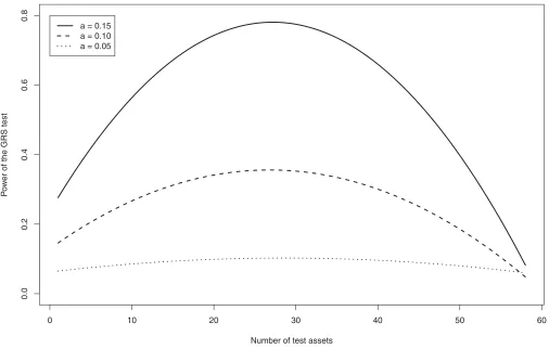
Figure 1. This figure plots the power of the GRS test as a function of the number of included test assets. The returns are generated from a one-factor model with normally distributed disturbances. The sample size isT =60 and the number of test assetsNranges from 1 to 58. The test is performed at a nominal 0.05 level. The higher power curves are associated with greater pricing errors.
The GRS test statistic is
J1=
T −N−K
N [1+¯f
′ˆ−1¯f
]−1ˆa′ˆ−1ˆa, (5)
whereˆ is given by
ˆ
= 1
T T
t=1
(ft−¯f)(ft−¯f)′.
Under the null hypothesisH0, the statisticJ1follows a central
Fdistribution withNdegrees of freedom in the numerator and (T −N−K) degrees of freedom in the denominator.
In practical applications of the GRS test, one needs to decide the appropriate numberNof test assets to include. It might seem natural to try to use as many as possible to increase the proba-bility of rejectingH0when it is false. As the test asset universe expands, it becomes more likely that nonzero pricing errors will be detected, if indeed there are any. However, the choice ofNis restricted byTto keep the estimate of the disturbance covariance matrix in (4) from becoming singular, and the choice ofTitself is often restricted owing to concerns about parameter stability. For instance, it is quite common to see studies whereT =60 monthly returns and N is between 10 and 30. The effects of increasing the number of test assets on test power are discussed in GRS, Campbell, Lo, and MacKinlay (1997, p. 206), and Sen-tana (2009). WhenN increases, three effects come into play: (i) the increase in the value of J1’s noncentrality parameter,
which increases power; (ii) the increase in the number of de-grees of freedom of the numerator, which decreases power; and (iii) the decrease in the number of degrees of freedom of the denominator due to the additional parameters that need to be estimated, which also decreases power.
To illustrate the net effect of increasingNon the power of the GRS test, we simulated model (1) withK=1, where the returns on the single factor are random draws from the standard normal distribution. The elements of the independent disturbance vector were also drawn from the standard normal distribution, thereby ensuring the exactness of the GRS test. We set T =60 and considered ai =0.05, 0.10, and 0.15, for i=1, . . . , N, and we let the number of test assets N range from 1 to 58. The chosen values forai are well within the range of what we find with monthly stock returns. Figure 1shows the power of the GRS test as a function ofN, where for any givenN, the higher power is associated with greater pricing errors. In line with the discussion in GRS, this figure clearly shows the power of the test given this specification rising asNincreases up to about one half of T, and then decreasing beyond that. The results in Table 5.2 of Campbell, Lo, and MacKinlay (1997) show several other alternatives against which the power of the GRS test declines asNincreases. Furthermore, there are no general results about how to devise an optimal multivariate test. So, great care must somehow be taken when choosing the number of test assets since power does not increase monotonically withN, and if the cross section is too large, then the GRS test may lose all its
power or may not even be computable. In fact, any procedure that relies on standard unrestricted estimates of the covariance matrix of regression disturbances will have this singularity problem whenNexceedsT.
3. TEST PROCEDURE
In this section, we develop a procedure to test exact factor pricing in the context of (1) that relaxes three assumptions of the GRS test: (i) the assumption of identically distributed distur-bances, (ii) the assumption of normally distributed disturdistur-bances, and (iii) the restriction thatN ≤T −K−1.
Our approach is motivated by a classical theorem in nonpara-metric statistics obtained in Lehmann and Stein (1949), which states that theonlytests which yield valid inference under suffi-ciently general distributional assumptions (allowing nonnormal, possibly heteroscedastic, independent observations) are ones that are conditional on the absolute values of the observations; that is, they must be based on sign statistics. Conversely, if a test procedure does not satisfy this condition for all levels 0< α <1, then its true size is 1 irrespective of its nominal size (Dufour2003).
3.1 Statistical Framework
As in the GRS framework, we assume that the disturbance vectorsεt in (1) are independently distributed over time, con-ditional onF. We do not require the disturbance vectors to be identically distributed, but we do assume that they satisfy a mul-tivariate symmetry condition each period. In what follows, the symbol=d stands for the equality in distribution.
Assumption 1. The cross-sectional disturbance vectors εt, for t=1, . . . , T, are mutually independent, continuous, and reflectively symmetric so thatεt
d
= −εt, conditional onF.
The distributions encompassed by this assumption include elliptically symmetric ones, such as the well-known multivariate normal (assumed by GRS) and Student’st distributions. The reflective symmetry condition in Assumption 1 is less stringent than elliptical symmetry. For instance, a mixture (finite or not) of distributions, each one elliptically symmetric around the origin, is not necessarily elliptically symmetric but it is reflectively symmetric.
Assumption 1 does not require the vectorsεtto be identically distributed nor does it restrict their degree of heterogeneity. This is a very attractive feature since it is well known that financial re-turns often depart quite dramatically from Gaussian conditions. In particular, the distribution of asset returns appears to have much heavier tails and is more peaked than a normal distribu-tion. The present framework leaves open not only the possibility of unknown forms of nonnormality, but also heteroscedastic-ity and time-varying covariances among the εt’s. For exam-ple, when (rt, ft) are elliptically distributed but nonnormal, the conditional covariance matrix ofεt depends on the contempo-raneous ft; see MacKinlay and Richardson (1991) and Zhou (1993). Here the disturbance covariance structure could be any function of the common factors (contemporaneous or not). The
simulation study in Section4examines a contemporaneous het-eroscedasticity specification.
3.2 Portfolio Formation
A usual practice in the application of the GRS test is to base it on portfolio groupings to haveNmuch less thanT. As Shanken (1996) noted, this has the potential effect of reducing the residual variances and increasing the precision with which
a=(a1, . . . , aN)′is estimated. On the other hand, as Roll (1979) emphasized, individual stock expected return deviations under the alternative can cancel out in portfolios, which would reduce the power of the GRS test unless the portfolios are combined in proportion to their weighting in the tangency portfolio. So ideally, all the pricing errors that make up the vectora in (1) would be of the same sign to avoid power losses when forming an equally weighted portfolio of the test assets.
Our approach here is an adaptive one based on a split-sample technique where the first subsample is used to obtain an estimate ofa. That estimate is then used to form a single portfolio that judiciously avoids power losses. Finally, a conditional test of exact factor pricing is performed using only the returns on that portfolio observed over the second subsample. This approach formalizes the usual practice of forming portfolios to deal with large N. It is important to note that our procedure does not introduce any of the data-snooping size distortions (i.e., the ap-pearance of statistical significance when the null hypothesis is true) discussed in Lo and MacKinlay (1990), since the estima-tion results are condiestima-tionally (on the factors) independent of the second subsample test outcomes.
LetT =T1+T2. In matrix form, the firstT1returns on asset
ican be represented by
r(1)i =aiι+F(1)bi+ε (1) i ,
where r(1)i =[ri1, . . . , riT1] ′
and F(1)=
[f1, . . . , fT1] ′
collect the time series ofT1returns on assetiand the factors, respec-tively,ιis a conformable vector of ones,b′
i is theith row ofB in (1), andε(1)i =[εi1, . . . , εiT1]
′.
Restriction 1. Only the firstT1 observations onrtandft are used to compute ˆa1, . . . ,aˆN.
This restriction does not limit the choice of estimation method, so the estimates ˆa1, . . . ,aˆNcould be obtained by OLS or any other method. Of course,T1must at least be enough to obtain the subsample estimates ˆa1, . . . ,aˆN. A well-known prob-lem with OLS though is that it is very sensitive to the presence of large disturbances and outliers; see Section5for evidence. An alternative estimation method is to minimize the sum of the ab-solute deviations in computing the regression lines (Bassett and Koenker1978). The resulting least absolute deviations (LAD) estimator may be more efficient than OLS in heavy-tailed sam-ples where extreme observations are more likely to occur. The results reported below in the simulation study and the empirical application are based on LAD.
With the estimatesaˆ =( ˆa1, . . . ,aˆN)′in hand, a vector of sta-tistically motivated “portfolio” weightsωˆ =( ˆω1,ωˆ2, . . . ,ωˆN)′
is computed according to returns on a portfolio computed asyt =
N
i=1ωˆirit,t =T1+ 1, . . . , T. We shall first provide a distributional result forytthat holds underH0and then explain in what sense the weights in (6) will maximize the power of the proposed distribution-free tests. In the following,δ=Ni=1ωˆiaiis the sum of the weightedai’s over the second subsample.
Proposition 1. UnderH0in (3) and when Assumption 1 and Restriction 1 hold,yt is represented by the single equation
yt=δ+f′tβ+ut, fort =T1+1, . . . , T , (7)
where δ =0 and (uT1+1, . . . , uT) d
=(±|uT1+1|, . . . ,±|uT|), conditional onF.
Proof. See the online Appendix (supplementary
materi-als).
The construction of a test based on a single portfolio group-ing is reminiscent of a mean-variance efficiency test proposed by Bossaerts and Hillion (1995) based onι′aˆ and another one proposed by Gungor and Luger (2009) that implicitly exploits
ι′a
. These approaches can suffer power losses depending on whether theai’s tend to cancel out when summed. Splitting the sample and applying the weights in (6) when forming the port-folio offsets that problem. Of course, if one believes a priori that theai’s do not tend to cancel out, then there is no need to split the sample and the test can proceed simply withωi =1/N.
The portfolio weights in (6) are in fact optimal in a cer-tain sense. To see how, recall thatεt is assumed to have well-defined first and second moments satisfying E[εt|ft]=0and E[εtε′t|ft]=t. Assumption 1 then implies that the mean and median (point of symmetry) coincide at zero for any com-ponent of εt. The power of our test procedure depends on E[ω′rt−ω′Bft|ft]=ω′a. (The next section shows how we deal with the presence of the nuisance parameters comprising
ω′B
.) As in the usual mean-variance portfolio selection prob-lem, choosingωto increaseω′a
also entails an increase in the portfolio’s varianceω′
tω, which decreases test power. So the problem we face is to maximizeω′asubject to a target value for
the variance. Here we set the target toι′
tι/N2, the variance of the naive, equally weighted portfolio that simply allocates equally across theNassets. It is easy to see thatω=sign(a)/N
will maximize power while keeping the resulting portfolio vari-ance as close as possible to the target. Of course, sign(a) is unknown, so (6) uses sign(aˆ). The possible discrepancy be-tween the achieved and the target variance values is given by
2 the off-diagonal (covariance) terms oft but not on any of its diagonal (variance) terms. Note that in an approximate APT factor model, these off-diagonal terms tend to zero asN → ∞. The weights in (6) are quite intuitive and represent the opti-mal choice in our distribution-free context where possible forms of distribution heterogeneity (e.g., time-varying variances and covariances) are left completely unspecified. Note that opti-mal weights in a strict mean-variance sense cannot be used here since finding these requires an estimate of the (possibly
time-varying) covariance structure and that is precisely what we are trying to avoid.
3.3 Test Statistics
The model in (7) can be represented in matrix form as
y=δι+F(2)β+u ements ofu follow what Coudin and Dufour (2009) called a “mediangale,” which is similar to the usual martingale differ-ence concept except that the median takes the place of the ex-pectation. The following result is an immediate consequence of the strict conditional mediangale property in Proposition 2.1 of Coudin and Dufour. Here we defines[x]=1, ifx ≥0, and
s[x]= −1, ifx <0.
Proposition 2. When Assumption 1 and Restriction 1 hold, theT2disturbance sign vector
s(y−δι−F(2)β)
=s[yT1+1−δ− f′T1+1β], . . . , s[yT −δ− f′Tβ] ′
follows a distribution free of nuisance parameters, conditional onF(2). Its exact distribution can be simulated to any degree of accuracy simply by repeatedly drawing ˜ST2 =(˜s1, . . . ,s˜T2)
′
whose elements are independent Bernoulli variables such that Pr[˜st =1]=Pr[˜st = −1]=1/2.
A corollary of this proposition is that any function of the disturbance sign vector and the factors, say =(s(y−δι−
F(2)β);F(2)), is also pivotal, conditional onF(2). To see the use-fulness of this result, consider the problem of testing
H0(δ0,β0) :δ=δ0,β=β0, (8) where δ0 andβ0 are specified values. Following Coudin and Dufour, we consider two test statistics for (8) given by the quadratic forms
nally onto the subspace spanned by the columns ofX. Boldin, Simonova, and Tyurin (1997) showed that these statistics can be associated with locally most powerful tests in the case of iid disturbances under some regularity conditions, and Coudin and Dufour extended this proof to more general disturbances that are not necessarily iid, but only satisfy the mediangale property. The statistic in (9) can be interpreted as a sign-based GMM statistic that exploits the property that each element of s(yt−δ0− f′tβ0)[1, f′t]
′
is a conditional mediangale un-derH0(δ0,β0). Note also that (10) can be interpreted as a sign analog of the usualF-test for testing the hypothesis that all the coefficients in a regression ofs(y−δ0ι−F(2)β0) onXare zero.
ST2′ P(X) ˜ST2, respectively. This means that appropriate critical values from the conditional distributions may be found to ob-tain finite-sample tests ofH0(δ0,β0). For instance, consider the statistic in (10). The decision rule is then to rejectH0(δ0,β0) at
levelαif SP(δ0,β0) is greater than the (1−α) quantile of the distribution obtained by simulatingSP, say cSP
α . (A critical value cSX
α can be found in a similar fashion by simulating valuesSX.) When (9) and (10) are evaluated at the true parameter values
δ andβ, Proposition 2 implies that Pr[SX(δ,β)> cSXα ]=α, and Pr[SP(δ,β)> cSPα ]=αas well. So, for all 0< α <1, the critical regions{SX(δ0,β0)> cSXα }and{SP(δ0,β0)> cSPα }each have sizeα. Note also that the critical valuescSXα andcSPα only need to be computed once, since they do not depend onδ0and
β0in (8).
Here the value of interest isδ0 =0, which means that we are dealing with point null hypotheses of the form
H0(β0) :δ=0,β=β0, (11)
whereβ0∈B, a set of admissible parameter values forβ. The null hypothesis implied by (3) that we wish to test is
H0p : β0∈B
H0(β0), (12)
the union of (11) taken overB. To test such a hypothesis, we appeal to aminimaxargument that may be stated as “reject the null whenever for all admissible values of the nuisance param-eters under the null, the corresponding point null hypothesis is rejected”; see Savin (1984). In general, this rule consists of maximizing thep-value of the sample test statistic over the set of nuisance parameters. Here it amounts to minimizing the values of the SX and SP statistics overB. To see why, define
SXL= inf
which shows that SPLis boundedly pivotal. This property further implies underH0pthat
PrSPL> cSPα
≤PrSP(0,β)> cαSP=α.
In other words, the test that rejects the null hypothesis H0p
whenever SPL> cSPα has levelα. The same argument applies to (9) to get the critical region SXL> cSXα .
We compute SXL and SPL in (13) by searching over a grid B(βˆ) specified around LAD point estimatesβˆ, which are com-puted in the restricted (i.e., no intercept) median regression modely=F(2)β+u
. Of course, more sophisticated optimiza-tion methods such as simulated annealing could be used to find SXLand SPL. The advantage of the naive grid search is that it is completely reliable and feasible when the dimension ofβis not too large. An important remark is that the search for SXL and SPL can be stopped and the null hypothesis can no longer be rejected at levelαas soon as a grid point yields a nonrejection. For instance, if SP(0,βˆ)≤cSP
α , then SPLdoes not reject either andH0pin (12) is not significant at levelα.
3.4 Summary of Test Procedure
Suppose one wishes to use the SPL statistic in (13). In a preliminary step, the reference distribution for this statistic is simulated to the desired degree of accuracy by generating a large number, sayM, of simulated iid valuesSP1, . . . ,SPM and
theα-level critical valuecSPα is determined from the simulated distribution. The rest of the test procedure then proceeds ac-cording to the following steps:
This procedure yields a distribution-free test in the sense that it remains exact over the class of all disturbance distributions satisfying Assumption 1. Note that the procedure is conditional on the factors, meaning that the critical valuecSP
α can only be obtained after the data have been observed.
4. SIMULATION EVIDENCE
We present the results of some simulation experiments to compare the performance of the proposed test procedure with several standard tests. The first of the benchmarks for compar-ison purposes is the GRSJ1test in (5). The other benchmarks are the usual LR test (J2), an adjusted LR test (J3) suggested by Jobson and Korkie (1982), and a test based on GMM (J4) proposed by MacKinlay and Richardson (1991). The latter is a particularly important benchmark here, since in principle it is robust to nonnormality and heteroscedasticity of returns. We also include in our comparisons two distribution-free tests (SD and WD) developed by Gungor and Luger (2009) that are ap-plicable even ifNis large, but only for the single-factor case. Details about all these tests are given in the online Appendix (supplementary materials).
The model specification that we examine is given by
rit =ai+bi1f1t+bi2f2t+bi3f3t+εit,
fort =1, . . . , T , i=1, . . . , N, (14)
with common factor returns following independent stochastic volatility processes of the form
fj t =exp(hj t/2)ǫj t, withhj t =λjhj,t−1+ξj t,
where the independent termsǫj t andξj tare both iid according to a standard normal distribution and the persistence parameters
λj are set to 0.5. The disturbances in (14) are subject to contem-poraneous heteroscedasticity of the formεit =exp(λift∗/2)ηit, where the innovationsηit are standard normal and theλi’s are randomly drawn from a uniform distribution between 1.5 and 2.5. We set f∗
t =(f1t+f2t+f3t)/3 so that all three factors
contribute equally to the variance heterogeneity; in the single-factor version (bi2=bi3=0), we set ft∗ =f1t. It should be noted that such a contemporaneous heteroscedastic specifica-tion finds empirical support in Duffee (1995,2001) and it is easy to observe that it generatesεit’s with time-varying excess kurtosis—a well-known feature of asset returns. The bij’s in (14) are randomly drawn from a uniform distribution between 0.5 and 1.5. All the tests are conducted at the nominal 5% level and critical values for SXLand SPLare determined using M=10,000. In the experiments, we choose mispricing values
aand set half the intercept values asai =aand the other half as ai= −a. We denote this in the tables as|ai| =a. The estimates of ai,i=1, . . . , N, in Step 1 of the procedure are found via LAD. Finally, each experiment comprises 1000 replications.
In the application of the test procedure, a choice needs to be made about where to split the sample. While this choice has no effect on the level of the tests, it obviously matters for their power. We do not have analytical results on how to split the sam-ple, so we resort to simulations. Overall, the results presented in the online Appendix (see the supplementary materials) suggest that no less that 30% and no more than 50% of the time-series observations should be used as the first subsample to maximize power. Accordingly, we pursue the testing strategy represented byT1=0.4T.
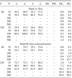
Tables 1 and 2 show the empirical size (Panel A) and power (Panel B) of the considered tests when|ai| =0.15 and T =60,120 andN takes on values between 10 and 500. The
Table 1. Empirical size and power: one-factor model
T N J1 J2 J3 J4 SD WD SXL SPL 100 73.8 73.8 73.8 65.3 89.6 95.3 52.3 60.1
200 – – – – 99.0 99.6 78.6 84.1
NOTES: This table reports the empirical size (Panel A) and size-corrected power (Panel B) of the GRS test (J1), the LR test (J2), an adjusted LR test (J3), a GMM-based test (J4), a sign test (SD), a Wilcoxon signed-rank test (SD), and the proposed SXLand SPL
tests. The returns are generated according to a single-factor model with contemporaneous heteroscedastic disturbances. The pricing errors are zero under the null hypothesis, whereas N/2 pricing errors are set equal to−0.15 and the other half are set to 0.15 under the alternative. The nominal level is 0.05 and entries are percentage rates. The results are based on 1000 replications and the symbol “–” is used whenever a test is not computable.
Table 2. Empirical size and power: three-factor model
T N J1 J2 J3 J4 SD WD SXL SPL
NOTES: This table reports the empirical size (Panel A) and size-corrected power (Panel B) of the GRS test (J1), the LR test (J2), an adjusted LR test (J3), a GMM-based test (J4), a sign test (SD), a Wilcoxon signed-rank test (SD), and the proposed SXLand SPL
tests. The returns are generated according to a three-factor model with contemporaneous heteroscedastic disturbances. The pricing errors are zero under the null hypothesis, whereas N/2 pricing errors are set equal to−0.15 and the other half are set to 0.15 under the alternative. The nominal level is 0.05 and entries are percentage rates. The results are based on 1000 replications and the symbol “–” is used whenever a test is not computable.
chosen value for|ai|is well within the range found in our em-pirical application, where the intercepts estimated with monthly stock returns range in values from−0.5 to 1.5. When they do not respect the nominal level constraint, the power results for theJtests are based on size-corrected critical values. It is im-portant to emphasize that size-corrected tests are not feasible in practice, especially under the very general symmetry condi-tion in Assumpcondi-tion 1. They are merely used here as theoretical benchmarks for the truly distribution-free tests. In particular, we wish to see how the power of the new tests compares with these benchmarks asT andN vary. Recall that the parametric tests are not computable whenNexceedsT; these cases are indicated with “–” in the tables.
Panel A of Tables1and2reveals that all the parametricJtests have massive size distortions, and these overrejections worsen asN increases for a givenT. The sensitivity of the GRS test to contemporaneous heteroscedasticity is also documented in MacKinlay and Richardson (1991), Zhou (1993), and Gungor and Luger (2009). WhenT =120 andN =10, theJtests all have empirical sizes around 20%. The probability of a Type I error for all these tests exceeds 65% whenN is increased to 50. In sharp contrast, the four distribution-free tests satisfy the nominal 5% level constraint, no matterT andN. In Panel B, we see the same phenomenon as in Figure 1: for a fixedT, the power of the GRS J1 test rises and then eventually drops as
Nkeeps on increasing. Note thatJ1,J2, andJ3 have identical size-corrected powers, since they are all related via monotonic
transformations (Campbell, Lo, and MacKinlay1997, Chap. 5). In contrast, the power of the SD and WD tests, as well as that of the new SXLand SPLtests, increases monotonically withN. At this point, one may wonder what is the advantage of the new SXL and SPL tests over the SD and WD tests of Gungor and Luger (2009) since the latter display better power in Panel B ofTable 1. These tests achieve higher power because they eliminate thebi1’s from the inference problem through the use of long differences, whereas the new tests proceed through a minimization of the test statistics over the intervening nuisance parameter space. A limitation of the SD and WD tests, how-ever, is that they are valid only under the assumption that the single-factor model disturbances are cross-sectionally indepen-dent. The online Appendix (see the supplementary materials) reports additional simulation results showing that the SD and WD tests are fairly robust to mild cross-sectional correlation, but start overrejecting as the cross-sectional dependence increases and this problem is further exacerbated asNincreases. Empir-ical sizes are also reported when the model disturbances are asymmetric, and the SXL and SPL tests are found to be quite robust to departures from symmetry.
Note also thatTable 2has no results for the SD and WD tests, since they are not computable in the presence of multiple factors. The overall pattern inTable 2echoes the previous findings for theJ tests about their size distortions and diminishing power as N increases. What is new inTable 2 is that the SXL and SPLtests appear generally more conservative, soNneeds to be increased further to attain the power levels seen inTable 1. In the empirical illustration that follows, we apply the new tests withN =10,100, and 503 test assets.
5. EMPIRICAL ILLUSTRATION
In this section, we illustrate the new tests with two empirical applications. First, we examine the Sharpe–Lintner version of the CAPM. This single-factor model uses the excess returns of a value-weighted stock market index of all stocks listed on the New York Stock Exchange (NYSE), American Stock Exchange (AMEX), and National Association of Securities Dealers Au-tomated Quotations (NASDAQ) markets. Second, we test the more general three-factor model of Fama and French (1993), which adds two factors to the CAPM specification: (i) the aver-age return on three small market capitalization portfolios minus the average return on three big market capitalization portfolios, and (ii) the average return on two value portfolios minus the average return on two growth portfolios. Note that the CAPM is nested within the Fama–French model. This means that if there was no sampling uncertainty, finding that the market portfolio is mean-variance efficient would trivially imply the validity of the three-factor model. Conversely, if the three-factor model does not hold, then the CAPM is also rejected.
We test both specifications with three sets of test assets com-prising the stocks traded on the NYSE, AMEX, and NASDAQ markets for the 38-year period from January 1973 to December 2010 (456 months). The first two datasets are the monthly re-turns on 10 portfolios formed on size, and 100 portfolios formed on both size and the book-to-market ratio. These two datasets are available in Ken French’s online data library. The third dataset comprises the returns on 503 individual stocks traded on the
markets mentioned above. These represent all the stocks for which there is data in the Center for Research in Security Prices (CRSP) monthly stock files for the entire 38-year sample period. Finally, we use the 1-month U.S. Treasury bill as the risk-free asset.
The full sample period contains several extreme observa-tions. For instance, the returns during the stock market crash of October 1987 and the financial crisis of 2008 are obviously not representative of normal market activity; we discuss the effects of extreme observations in Section 5.3. It is also quite com-mon in the empirical finance literature to perform asset pricing tests over subperiods out of concerns about parameter stability. So, in addition to the entire 38-year period, we also examine six 5-year, one 8-year, and three 10-year subperiods. For other examples of this practice, see Campbell, Lo, and MacKinlay (1997), Gungor and Luger (2009), and Ray, Savin, and Tiwari (2009). Here we present the results based on the 10 size port-folios and 503 individual stocks, while those based on the 100 size and book-to-market portfolios are reported in the online Appendix (see the supplementary materials).
5.1 10 Size Portfolios
Table 3reports the CAPM test results based on the 10 size portfolios. The numbers reported in parenthesis are p-values and the entries in bold represent cases of significance at the 5% level. We observe that the parametricJtests reject the null hypothesis over the entire sample period withp-values no more than 5%. The nonparametric SD and WD tests also indicate strong rejections. In contrast, the SXLand SPLtests clearly do not reject the mean-variance efficiency of the market index.
Looking at the subperiods, we observe that the only rejec-tion by the new tests occurs with SPLin the 10-year subperiod 1/73–12/82. In the 5-year subperiod 1/98–12/02, theJ2andJ4 tests reject the CAPM specification. The results for theJtests during the last 10-year subperiod from 1/93 to 12/02 agree with the rejection findings for the entire sample period. Besides the obvious differences between the parametric and the nonpara-metric inference results,Table 3also reveals some differences between the SD and WD tests and the proposed SXLand SPL tests. One possible reason for the disagreement across these nonparametric tests could be the presence of cross-sectional disturbance correlations. Indeed, the SD and WD tests are not invariant to such correlations, whereas the new tests allow for cross-sectional dependencies just like the GRS test.
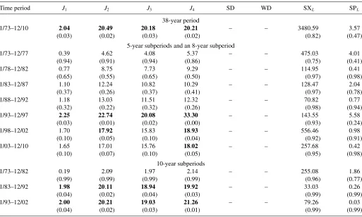
Table 4shows the results for the Fama–French model. For the entire 38-year sample period, the results in Table 4are in line with those for the single-factor model inTable 3. The stan-dardJtests reject the null with very lowp-values, whereas the distribution-free SXL and SPL tests are not significant. In the 5-year subperiods, we see some disagreements among the para-metric tests. For instance, during 1/98–12/02, theJ1andJ3tests indicate nonrejections, whileJ2andJ4point toward rejections of the null. The results for the last two 10-year subperiods re-semble those for the entire sample period and theJtests depict a more coherent picture.
Table 4shows that the SXL and SPL tests never reject the three-factor specification. Taken at face value, these results would suggest that the excess returns of the 10 size portfolios
Table 3. Tests of the CAPM with 10 size portfolios
Time period J1 J2 J3 J4 SD WD SXL SPL
38-year period
1/73–12/10 1.83 18.43 18.14 18.48 38.45 35.25 208.77 0.06
(0.05) (0.05) (0.05) (0.04) (0.00) (0.00) (0.92) (0.97)
5-year subperiods and an 8-year subperiod
1/73–12/77 0.56 6.46 5.71 5.24 16.80 15.09 197.79 4.02
(0.83) (0.77) (0.84) (0.87) (0.08) (0.12) (0.64) (0.14)
1/78–12/82 1.12 12.38 10.93 10.90 54.93 42.28 204.06 3.77
(0.36) (0.26) (0.36) (0.37) (0.00) (0.00) (0.69) (0.16)
1/83–12/87 0.81 9.20 8.12 8.75 5.46 5.14 128.48 1.24
(0.62) (0.51) (0.61) (0.55) (0.85) (0.88) (0.81) (0.55)
1/88–12/92 0.79 9.01 7.96 8.13 21.60 10.83 16.98 0.22
(0.63) (0.53) (0.63) (0.62) (0.01) (0.37) (0.94) (0.89)
1/93–12/97 1.08 12.00 10.60 12.64 2.26 1.85 37.58 0.72
(0.39) (0.29) (0.38) (0.24) (0.99) (0.99) (0.86) (0.69)
1/98–12/02 1.87 19.43 17.16 18.66 4.93 2.85 100.96 1.00
(0.07) (0.03) (0.07) (0.04) (0.89) (0.98) (0.82) (0.63)
1/03–12/10 1.73 17.84 16.54 17.45 10.16 7.37 45.42 0.03
(0.09) (0.06) (0.09) (0.06) (0.42) (0.68) (0.93) (0.98)
10-year subperiods
1/73–12/82 0.73 7.85 7.39 7.49 46.00 60.16 1298.92 15.01
(0.69) (0.64) (0.68) (0.67) (0.00) (0.00) (0.38) (0.00)
1/83–12/92 1.48 15.29 14.40 14.59 11.00 8.30 112.25 0.54
(0.15) (0.12) (0.15) (0.14) (0.36) (0.60) (0.87) (0.77)
1/93–12/02 2.07 20.93 19.71 20.17 4.60 3.84 146.37 1.06
(0.03) (0.02) (0.03) (0.02) (0.92) (0.95) (0.85) (0.58)
NOTES: The results are based on value-weighted returns of 10 portfolios formed on size. The market portfolio is the value-weighted return on all NYSE, AMEX, and NASDAQ stocks and the risk-free rate is the 1-month Treasury bill rate. The numbers in parentheses arep-values and entries in bold represent cases of significance at the 5% level.
Table 4. Tests of the Fama–French model with 10 size portfolios
Time period J1 J2 J3 J4 SD WD SXL SPL
38-year period
1/73–12/10 2.04 20.49 20.18 20.21 – – 3480.59 3.57
(0.03) (0.02) (0.03) (0.02) (0.82) (0.47)
5-year subperiods and an 8-year subperiod
1/73–12/77 0.39 4.62 4.08 5.37 – – 475.03 4.01
(0.94) (0.91) (0.94) (0.86) (0.75) (0.41)
1/78–12/82 0.77 8.75 7.73 9.29 – – 114.95 0.41
(0.65) (0.55) (0.65) (0.50) (0.97) (0.98)
1/83–12/87 1.10 12.24 10.82 10.29 – – 128.47 2.04
(0.37) (0.26) (0.37) (0.41) (0.97) (0.78)
1/88–12/92 1.18 13.03 11.51 12.32 – – 70.82 0.77
(0.32) (0.22) (0.32) (0.26) (0.98) (0.94)
1/93–12/97 2.25 22.74 20.08 33.30 – – 143.55 5.58
(0.03) (0.01) (0.02) (0.00) (0.93) (0.24)
1/98–12/02 1.70 17.92 15.83 18.93 – – 556.46 0.98
(0.10) (0.05) (0.10) (0.04) (0.92) (0.91)
1/03–12/10 1.65 17.01 15.76 18.02 – – 257.68 0.42
(0.10) (0.07) (0.10) (0.05) (0.95) (0.98)
10-year subperiods
1/73–12/82 0.19 2.09 1.97 2.14 – – 255.08 1.86
(0.99) (0.99) (0.99) (0.99) (0.96) (0.77)
1/83–12/92 1.98 20.11 18.94 19.92 – – 33.03 0.26
(0.04) (0.02) (0.04) (0.03) (0.99) (0.99)
1/93–12/02 2.00 20.21 19.03 21.26 – – 79.26 0.03
(0.04) (0.02) (0.03) (0.01) (0.99) (0.99)
NOTES: The results are based on value-weighted returns of 10 portfolios formed on size, the returns on the three Fama–French factors, and the 1-month Treasury bill rate as the risk-free rate. The numbers in parentheses arep-values and entries in bold represent cases of significance at the 5% level. The symbol “–” is used whenever a test is not computable.
are well explained by the three Fama–French factors. This is entirely consistent with the nonrejections seen inTable 3 and it suggests that the size and the book-to-market factors play no role; that is, the CAPM factor alone can price the 10 size portfolios.
Upon observing that the Fama–French model is never rejected by the nonparametric SXLand SPLtests with 10 test assets, one may be concerned about the ability of the new procedure to reject the null when the alternative is true. To boost power, we proceed next with a 50-fold increase in the number of test assets.
5.2 503 Individual Stocks
Tables5and6report the test results using the returns on 503 individual stocks. Here theJ tests cannot be computed, since
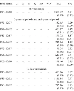
N > T. When compared to the test outcomes with the 100 size and book-to-market portfolios (reported in the online Ap-pendix), the most striking result is that now for the entire sample period (T =456), the preferred SPL test no longer indicates a rejection of either the CAPM nor the Fama–French three-factor model. The SD and WD tests also agree with the nonrejection of the CAPM when moving from those 100 portfolios to individual stocks.
These results suggest that the excess returns on individual stocks are well explained by the CAPM, which in turn suggests
Table 5. Tests of the CAPM with 503 individual stocks
Time period J1 J2 J3 J4 SD WD SXL SPL
38-year period
1/73–12/10 – – – – 478.26 483.68 696.34 2.03 (0.78) (0.72) (0.79) (0.36)
5-year subperiods and an 8-year subperiod
1/73–12/77 – – – – 466.13 436.72 242.51 6.22 (0.87) (0.98) (0.59) (0.04) 1/78–12/82 – – – – 566.26 522.36 106.39 0.66
(0.02) (0.26) (0.80) (0.72) 1/83–12/87 – – – – 492.53 504.74 20.79 0.31
(0.62) (0.46) (0.95) (0.86) 1/88–12/92 – – – – 496.40 500.58 35.88 0.05
(0.57) (0.52) (0.90) (0.97) 1/93–12/97 – – – – 418.13 432.12 10.76 0.11
(0.99) (0.99) (0.95) (0.95) 1/98–12/02 – – – – 429.46 353.28 205.36 4.74
(0.99) (1.00) (0.71) (0.09) 1/03–12/10 – – – – 497.16 484.88 200.58 1.85
(0.56) (0.71) (0.78) (0.40)
10-year subperiods
1/73–12/82 – – – – 594.33 600.21 201.15 2.55 (0.00) (0.00) (0.78) (0.28) 1/83–12/92 – – – – 511.40 503.47 28.39 0.24
(0.38) (0.48) (0.96) (0.88) 1/93–12/02 – – – – 538.13 481.90 199.84 2.72
(0.13) (0.74) (0.81) (0.26)
NOTES: The results are based on the returns of 503 individual stocks traded on the NYSE, AMEX, and NASDAQ markets. The market portfolio is the value-weighted return on all NYSE, AMEX, and NASDAQ stocks and the risk-free rate is the 1-month Treasury bill rate. The numbers in parentheses arep-values and entries in bold represent cases of significance at the 5% level. The symbol “–” is used whenever a test is not computable.
Table 6. Tests of the Fama–French model with 503 individual stocks
Time period J1 J2 J3 J4 SD WD SXL SPL
38-year period
1/73–12/10 – – – – – – 2387.42 6.71
(0.89) (0.15)
5-year subperiods and an 8-year subperiod
1/73–12/77 – – – – – – 182.15 0.29
(0.93) (0.99)
1/78–12/82 – – – – – – 463.17 2.49
(0.81) (0.67)
1/83–12/87 – – – – – – 191.72 1.87
(0.95) (0.81)
1/88–12/92 – – – – – – 246.14 1.12
(0.88) (0.90)
1/93–12/97 – – – – – – 90.24 0.52
(0.96) (0.97)
1/98–12/02 – – – – – – 642.42 2.61
(0.91) (0.65)
1/03–12/10 – – – – – – 149.46 0.15
(0.98) (0.99)
10-year subperiods
1/73–12/82 – – – – – – 483.76 0.87
(0.89) (0.93)
1/83–12/92 – – – – – – 1165.84 0.77
(0.68) (0.94)
1/93–12/02 – – – – – – 775.66 0.73
(0.93) (0.95)
NOTES: These results are based on the returns of 503 individual stocks traded on the NYSE, AMEX, and NASDAQ markets, the returns on the three Fama–French factors, and the 1-month Treasury bill rate as the risk-free rate. The numbers in parentheses arep-values and entries in bold represent cases of significance at the 5% level. The symbol “–” is used whenever a test is not computable.
that the size and book-to-market factors play no role in pricing this collection of assets. It also appears that creating portfolios on the basis of size and book-to-market biases the test outcomes toward a rejection of the model’s validity. This finding with the newly proposed SPLtest is entirely consistent with the analysis in Lo and MacKinlay (1990), who showed that sorting stocks into groups based on variables that are correlated with returns is a questionable practice since it favors a rejection of the asset pricing model under consideration; see also Berk (2000) for related theoretical analysis. Finally, it is interesting to note that this conclusion about the validity of the CAPM is also reached by Zhou (1993), Vorkink (2003), Gungor and Luger (2009), and Ray, Savin, and Tiwari (2009).
5.3 Extreme Observations
Looking back upon the results in Tables 3 and 4 with 10 size portfolios, one might think that the differences between the parametricJtests and the SXLand SPLtests are due to a lack of power by the latter whenNis small. Yet another plausible reason for these differences is the adverse effect that a small number of extreme observations can have on the OLS estimates used to compute theJtests; see Vorkink (2003). To investigate this possibility, we recompute the parametric tests with Winsorized data. This procedure has the effect of decreasing the magnitude
Table 7. Sensitivity of parametric tests to extreme observations
0% 0.3% 0.5% 0.7% 1.0%
Panel A: CAPM
J1 1.83 1.54 0.89 0.64 0.59
(0.05) (0.12) (0.54) (0.77) (0.81)
J2 18.43 15.55 9.05 6.54 6.07
(0.05) (0.11) (0.52) (0.76) (0.80)
J3 18.14 15.31 8.91 6.44 5.97
(0.05) (0.12) (0.54) (0.77) (0.81)
J4 18.48 14.94 8.12 6.11 5.82
(0.04) (0.13) (0.61) (0.80) (0.83)
Panel B: Fama–French model
J1 2.04 1.70 0.87 0.59 0.55
(0.03) (0.07) (0.55) (0.81) (0.85)
J2 20.49 17.13 8.91 6.05 5.63
(0.02) (0.07) (0.54) (0.81) (0.84)
J3 20.18 16.86 8.77 5.96 5.54
(0.03) (0.07) (0.55) (0.82) (0.85)
J4 20.21 16.31 8.16 5.63 5.10
(0.02) (0.09) (0.61) (0.84) (0.88)
NOTES: This table shows the results of the parametric tests with the 10 size portfolios when the returns for the full sample period from January 1973 to December 2010 are Winsorized at various small levels. Panels A and B correspond to the one- and three-factor models, respectively. The numbers in parenthesis arep-values and bold entries represent cases of significance at the 5% level.
of extreme observations but leaves them as important points in the sample.
Table 7 shows the results of the J tests with the 10 size portfolios when the full sample returns are Winsorized at the 0.3%, 0.5%, 0.7%, and 1% levels. In the single-factor case (Panel A), theJtests cease to be significant at the 5% level with returns Winsorized at 0.3%. For the three-factor model (Panel B), the same pattern of increasingp-values occurs across Winsorization levels. These results clearly show that OLS-based inference can be very sensitive to the presence of even just a few extreme observations.
6. CONCLUSION
The beta-pricing representation of linear factor pricing mod-els is typically assessed with tests based on OLS or GMM. In this context, standard asymptotic theory is known to provide a poor approximation to the finite-sample distribution of those test statistics, even with fairly large samples. In particular, the asymptotic tests tend to overreject the null hypothesis when in fact it is true, and these size distortions grow quickly as the number of included test assets increases. So, the conclusions of empirical studies that adopt such procedures can lead one to spuriously reject the validity of the asset pricing model.
Exact finite-sample methods that avoid the spurious rejec-tion problem usually rely on strong distriburejec-tional assumprejec-tions about the model’s disturbance terms. A prominent example is the GRS test that assumes that the disturbances are identically distributed each period according to a multivariate normal distri-bution. Yet it is known from the empirical literature that financial asset returns are nonnormal, exhibiting time-varying covariance structures and excess kurtosis. These stylized facts would put into question the reliability of any inference method which
assumes that the cross-sectional distribution of disturbance terms is homogenous over time.
Another serious problem with standard inference methods has to do with the choice of how many test assets to include. Indeed, if too many are included relative to the number of available time-series observations, the GRS test may lose all its power or may not even be computable. In fact, any procedure that relies on unrestricted estimates of the covariance matrix of regression disturbances will no longer be computable owing to the singu-larity that occurs when the size of the cross section exceeds the length of the time series.
In this article, we have proposed a finite-sample test proce-dure that overcomes these problems. Specifically, our statistical framework makes no parametric assumptions about the distri-bution of the disturbance terms in the factor model. The only requirement is that the cross-sectional disturbance vectors be independent over time, conditional on the factors, and reflec-tively symmetric each period. The class of reflecreflec-tively symmet-ric distributions includes elliptically symmetsymmet-ric ones, which are theoretically consistent with mean-variance analysis. Our non-parametric framework leaves open the possibility of unknown forms of time-varying nonnormalities and many other distribu-tion heterogeneities, such as time-varying covariance structures, time-varying kurtosis, etc.
The procedure is an adaptive one that first splits the sample to combine the assets into a single portfolio using weights based on the signs of estimated regression intercepts from a subsample. This approach formalizes the usual practice of forming portfo-lios to solve the problem of too many test assets. Of course, it could also be used in conjunction with an assumed form of the multivariate disturbance distribution to devise a paramet-ric test. The Lehmann and Stein (1949) impossibility theorem, however, shows that if we wish to remain completely agnostic about heteroscedasticity, then the only valid tests are ones based on sign statistics. Even though some studies such as Affleck-Graves and McDonald (1989) report evidence showing the GRS test to be fairly robust to (some specified) deviations from nor-mality, we find it hard to have faith in a parametric procedure whose assumptions are so obviously at odds with the empiri-cal evidence. Moreover, our results show that the power of the new sign-based test procedure increases as either the time-series lengthens and/or the cross section becomes larger. So, the truly robust inference procedure developed here offers a very com-pelling way to assess the validity of linear factor pricing models, especially with a large number of test assets.
SUPPLEMENTARY MATERIALS
The online Appendix contains the proof of Proposition 1, details about the other tests used for comparison purposes, ad-ditional simulation evidence, and the empirical results for the 100 size and book-to-market portfolios.
ACKNOWLEDGMENTS
We thank Lynda Khalaf, Antonio Diez de los Rios, two anony-mous referees, an associate editor, and the editor Jonathan Wright for helpful comments. Earlier versions of this arti-cle were presented at Northern Illinois University, the 2010
Meetings of the Midwest Econometrics Group, the 2010 Inter-national Conference on “High-Dimensional Econometric Mod-elling” at Cass Business School, and the 2011 North American Summer Meeting of the Econometric Society. The views in this article are solely the responsibility of the authors and should not be interpreted as reflecting the views of the Bank of Canada.
[Received February 2012. Revised October 2012.]
REFERENCES
Affleck-Graves, J., and McDonald, B. (1989), “Nonnormalities and Tests of Asset Pricing Theories,”Journal of Finance, 44, 889–908. [66,76] Bassett, G., and Koenker, R. (1978), “Asymptotic Theory of Least Absolute
Error Regression,”Journal of the American Statistical Association, 73, 618– 622. [69]
Beaulieu, M.-C., Dufour, J.-M., and Khalaf, L. (2007), “Multivariate Tests of Mean-Variance Efficiency With Possibly Non-Gaussian Errors: An Exact Simulation-Based Approach,”Journal of Business and Economic Statistics, 25, 398–410. [66]
Berk, J. (2000), “Sorting Out Sorts,”Journal of Finance, 55, 407–427. [75] Blattberg, R., and Gonedes, N. (1974), “A Comparison of the Stable and Student
Distributions as Statistical Models of Stock Prices,”Journal of Business, 47, 244–280. [66]
Boldin, M. V., Simonova, G. I., and Tyurin, Y. N. (1997),Sign-Based Methods in Linear Statistical Models, Baltimore, MD: American Mathematical Society. [70]
Bossaerts, P., and Hillion, P. (1995), “Testing the Mean-Variance Efficiency of Well-Diversified Portfolios in Very Large Cross-Sections,” Annales d’ ´Economie et de Statistique, 40, 93–124. [70]
Campbell, J. Y., Lo, A. W., and MacKinlay, A. C. (1997),The Econometrics of Financial Markets, Princeton, NJ: Princeton University Press. [66,68,73] Chou, P.-H., and Zhou, G. (2006), “Using Bootstrap to Test Portfolio Efficiency,”
Annals of Economics and Finance, 1, 217–249. [66]
Coudin, E., and Dufour, J.-M. (2009), “Finite-Sample Distribution-Free Infer-ence in Linear Median Regressions Under Heteroscedasticity and Nonlin-ear Dependence of Unknown Form,”Econometrics Journal, 12, S19–S49. [67,70]
Duffee, G. R. (1995), “Stock Returns and Volatility: A Firm-Level Analysis,” Journal of Financial Economics, 37, 399–420. [72]
——— (2001), “Asymmetric Cross-Sectional Dispersion in Stock Returns: Evidence and Implications,” Working Paper No. 2000-18, Federal Reserve Bank of San Francisco. [72]
Dufour, J.-M. (2003), “Identification, Weak Instruments, and Statistical In-ference in Econometrics,” Canadian Journal of Economics, 36, 767– 808. [69]
Dufour, J.-M., and Khalaf, L. (2002), “Simulation Based Finite and Large Sample Tests in Multivariate Regressions,”Journal of Econometrics, 111, 303–322. [66]
Dufour, J.-M., and Taamouti, A. (2010), “Exact Optimal Inference in Regression Models Under Heteroskedasticity and Non-Normality of Unknown Form,” Computational Statistics and Data Analysis, 54, 2532–2553. [67] Fama, E. (1965), “The Behavior of Stock-Market Prices,”Journal of Business,
38, 34–105. [66]
Fama, E. F., and French, K. R. (1993), “Common Risk Factors in the Returns on Stocks and Bonds,”Journal of Financial Economics, 33, 3–56. [73] Ferson, W. E., and Foerster, S. R. (1994), “Finite Sample Properties of the
Generalized Method of Moments in Tests of Conditional Asset Pricing Models,”Journal of Financial Economics, 36, 29–55. [66]
Gibbons, M. R., Ross, S. A., and Shanken, J. (1989), “A Test of the Efficiency of a Given Portfolio,”Econometrica, 57, 1121–1152. [66]
Grinblatt, M., and Titman, S. (1987), “The Relation Between Mean-Variance Efficiency and Arbitrage Pricing,”Journal of Business, 60, 97–112. [67] Gungor, S., and Luger, R. (2009), “Exact Distribution-Free Tests of
Mean-Variance Efficiency,” Journal of Empirical Finance, 16, 816–829. [66,70,71,72,73,75]
Hsu, D. A. (1982), “A Bayesian Robust Detection of Shift in the Risk Structure of Stock Market Returns,”Journal of the American Statistical Association, 77, 29–39. [66]
Huberman, G., Kandel, S., and Stambaugh, R. F. (1987), “Mimicking Portfolios and Exact Arbitrage Pricing,”Journal of Finance, 42, 1–9. [67]
Jobson, J. D. (1982), “A Multivariate Linear Regression Test for the Arbitrage Pricing Theory,”Journal of Finance, 37, 1037–1042. [67]
Jobson, J. D., and Korkie, B. (1982), “Potential Performance and Tests of Portfolio Efficiency,”Journal of Financial Economics, 10, 433–466. [67,71] ——— (1985), “Some Tests of Linear Asset Pricing With Multivariate
Normal-ity,”Canadian Journal of Administrative Sciences, 2, 114–138. [67] Jouneau-Sion, F., and Torr`es, O. (2006), “MMC Techniques for Limited
De-pendent Variables Models: Implementation by the Branch-and-Bound Al-gorithm,”Journal of Econometrics, 133, 479–512. [67]
Kocherlakota, N. R. (1997), “Testing the Consumption CAPM With Heavy-Tailed Pricing Errors,”Macroeconomic Dynamics, 1, 551–567. [66] Lehmann, E. L., and Stein, C. (1949), “On the Theory of Some Non-Parametric
Hypotheses,”Annals of Mathematical Statistics, 20, 28–45. [67,69,76] Lintner, J. (1965), “The Valuation of Risk Assets and the Selection of Risky
Investments in Stock Portfolios and Capital Budgets,”Review of Economics and Statistics, 47, 13–37. [66,67]
Lo, A., and MacKinlay, A. C. (1990), “Data-Snooping Biases in Tests of Fi-nancial Asset Pricing Models,”Review of Financial Studies, 3, 431–467. [69,75]
MacKinlay, A. C., and Richardson, M. P. (1991), “Using Generalized Method of Moments to Test Mean-Variance Efficiency,”Journal of Finance, 46, 511–527. [66,69,71,72]
Merton, R. C. (1973), “An Intertemporal Capital Asset Pricing Model,” Econo-metrica, 41, 867–887. [66]
Newey, W. K., and West, K. D. (1987), “A Simple, Positive Semidefinite, Het-eroskedasticity and Autocorrelation Consistent Covariance Matrix,” Econo-metrica, 55, 703–708. [67]
Ray, S., Savin, N. E., and Tiwari, A. (2009), “Testing the CAPM Revisited,” Journal of Empirical Finance, 16, 721–733. [73,75]
Roll, R. (1979), “A Reply to Mayers and Rice (1979),”Journal of Financial Economics, 7, 391–400. [69]
Ross, S. A. (1976), “The Arbitrage Theory of Capital Asset Pricing,”Journal of Economic Theory, 13, 341–360. [66]
Savin, N. E. (1984), “Multiple Hypothesis Testing,” inHandbook of Economet-rics, eds. Z. Griliches and M. D. Intriligator, Amsterdam: North-Holland, pp. 827–879. [71]
Sentana, E. (2009), “The Econometrics of Mean-Variance Efficiency Tests: A Survey,”Econometrics Journal, 12, C65–C101. [68]
Shanken, J. (1987), “A Bayesian Approach to Testing Portfolio Efficiency,” Journal of Financial Economics, 19, 195–215. [67]
——— (1996), “Statistical Methods in Tests of Portfolio Efficiency: A Synthe-sis,” inHandbook of Statistics: Statistical Methods in Finance, eds. G. S. Maddala and C. R. Rao, Amsterdam: North-Holland, pp. 693–711. [66,69] Sharpe, W. F. (1964), “Capital Asset Prices: A Theory of Market Equilibrium
Under Conditions of Risk,”Journal of Finance, 19, 425–442. [66,67] Vorkink, K. (2003), “Return Distributions and Improved Tests of Asset Pricing
Models,”Review of Financial Studies, 16, 845–874. [75]
White, H. (1980), “A Heteroskedasticity-Consistent Covariance Matrix Esti-mator and a Direct Test for Heteroskedasticity,”Econometrica, 48, 817– 838. [67]
Zhou, G. (1993), “Asset-Pricing Tests Under Alternative Distributions,”Journal of Finance, 48, 1927–1942. [66,69,72,75]