Full Terms & Conditions of access and use can be found at
http://www.tandfonline.com/action/journalInformation?journalCode=ubes20
Download by: [Universitas Maritim Raja Ali Haji] Date: 13 January 2016, At: 00:26
Journal of Business & Economic Statistics
ISSN: 0735-0015 (Print) 1537-2707 (Online) Journal homepage: http://www.tandfonline.com/loi/ubes20
Spatial Modeling of House Prices Using
Normalized Distance-Weighted Sums of Stationary
Processes
S Banerjee, A. E Gelfand, J. R Knight & C. F Sirmans
To cite this article: S Banerjee, A. E Gelfand, J. R Knight & C. F Sirmans (2004) Spatial Modeling of House Prices Using Normalized Distance-Weighted Sums of Stationary Processes, Journal of Business & Economic Statistics, 22:2, 206-213, DOI: 10.1198/073500104000000091
To link to this article: http://dx.doi.org/10.1198/073500104000000091
View supplementary material
Published online: 01 Jan 2012.
Submit your article to this journal
Article views: 102
View related articles
Spatial Modeling of House Prices Using
Normalized Distance-Weighted Sums
of Stationary Processes
S. B
ANERJEEDivision of Biostatistics, University of Minnesota, Minneapolis, MN 55455
A. E. G
ELFANDInstitute of Statistics and Decision Sciences, Duke University, Durham, NC 27708-0251 (alan@stat.duke.edu)
J. R. K
NIGHTEberhardt School of Business, University of the Pacic, Stockton, CA 95211
C. F. S
IRMANSCenter for Real Estate and Urban Economic Studies, University of Connecticut, Storrs, CT 06269-1041
Hedonic models are used almost universally for modeling house prices. Recognizing the importance of location, the past decade has seen increasing effort to introduce spatial considerations into such modeling. When spatial process models are used to capture association between locations, isotropic specications have been used almost exclusively despite the fact that they seem unlikely to be appropriate in practice. The contribution of this article is to offer a novel, exible, and computationally tractable class of non-stationary models. We accomplish this using suitably normalized distance-weighted sums of non-stationary processes. The number of component processes used reects the exibility required to adequately explain the spatial residuals in the model. A exible nugget (or pure error) process is also introduced and is needed to capture the nonspatial idiosyncrasies of house sale transactions. The models are tted within a Bayesian framework requiring demanding computation but yielding full and exact inference through the posterior distributions of the model unknowns. A dataset of 656 single-family home sales in Stockton, California, provide an illustration.
1. INTRODUCTION
The literature on hedonic modeling for house prices is by now enormous; see, for example, the special issue of the Jour-nal of Real Estate Finance and Economics, January/March 1997, and further references therein. Recognizing the impor-tance of location in determining house price, the past decade has seen numerous articles which attempt to introduce spatial con-siderations into such modeling. The recent article by Gelfand, Ecker, Knight, and Sirmans (2004) provides a partial review of this work.
One widely used approach is to incorporate spatial features of the house location into the hedonic mean in addition to char-acteristics of the property. Such features might include an in-dicator variable for municipal or school district or a distance, such as to the central business district or a major highway. Still, there will always be characteristics which we do not know about or can not hope to measure. So, one could argue for a more parsimonious mean specication and, in the error specication, allow location to proxy for such omitted variables. More pre-cisely, this requires specifying spatial dependence in the resid-uals captured through the geocoded locations of the properties. The customary way to implement this approach is to model dependence between locations as a function of the distance be-tween them. Suchisotropicspecications seem unlikely to be appropriate in practice. Strength of spatial association would likely depend on where the pair of locations lies in the study re-gion, not just the distance between the locations. This requires prescription of a nonstationary spatial process model. Histor-ically, such models have resided in the theoretical probability
literature, with little concern for application. The contribution of this article is to propose a novel, exible, and computation-ally tractable class of nonstationary spatial models, to clarify its properties, and to show how such models may be tted in the context of a hedonic mean specication. We illustrate this using a dataset of selling prices for single-family homes in Stockton, California.
Looking at the modeling a bit more formally, a widely used specication is as follows (see, e.g., Cressie 1993, p. 112). Fors2D;Da region inR2, letY.s/denote the associated
re-sponse. Then setY.s/D¹.s/Cw.s/C².s/, where¹.s/is the
mean ofY.s/;typically of the formXT.s/¯;w.s/is a mean-0
stationary spatial Gaussian process; and².s/is a pure (white)
noise process. Again, the error structure associated with this model will be too restrictive for many applications.
We propose enriching both components of the error process. We extend the spatial component using a suitably normalized distance-weighted sum of stationary processes. The choice of weights introduceslocalstationarity into the specication in the spirit of Fuentes and Smith (2001) but with important structural differences. The resulting specication motivates the proposed pure error component model. This model is also specied in a local fashion, but now using indicator functions as weights. We claim that this is sensible, because pure error is not intended to reect distance. It is also necessary to enable adequate exibil-ity in the entire error model.
© 2004 American Statistical Association Journal of Business & Economic Statistics April 2004, Vol. 22, No. 2 DOI 10.1198/073500104000000091
206
Banerjee, et al.: Spatial Modeling of House Prices 207
As noted earlier, nonstationarity enables the intuitively ap-pealing possibility that both variability and the nature of spatial association depend on location in the region. Apart from the aforementioned work of Fuentes and Smith (2001), there have been other recent related works in this area, including that of Haas (1995), Higdon, Swall, and Kern (1999), and Agarwal, Gelfand, Sirmans, and Thibodean (2001).
The article of Agarwal et al. (2001), though similar in spirit, differs from the present article in several critical ways. First, we introduce the local nature through spatialknots, which we illustratively create through a rectangle partitioning approach. Agarwal et al. (2001) specied local regions based on an ex-ternal consideration, for example, market segmentation driven by economic considerations. They determined the number of regions as the number of submarkets (although aggregation is possible); each location belongs to a submarket. In contrast, we model the spatial error at each location as a unique weighted sum (where weights reect distance to knots) of independent but not identically distributed mean-0 normal variables. Lo-cations do not belong to submarkets; there is no notion of a submarket. Rather, we are modeling spatial error across the re-gion using a nonstationary process created through locally de-termined weighted sums of stationary processes. The number of components (equivalently, the number of knots) is exible. We use a model choice procedure to select the appropriate num-ber of knots. It is not of interest to explain this numnum-ber or the knot locations. Second, we use a particular normalization of our weights so that global stationarity becomes an extreme case. In contrast, Agarwal et al. (2001) intentionally“tuned” the weights so that inuence drops off rapidly in distance, with the result that local behavior dominates. In fact, they introduced an approximation for model tting that enables (conditional) inde-pendence of the models across the local regions. Finally, based on the segmentation of the region, Agarwal et al. (2001) in-troduced spatially varying coefcients. We focus on the error structure. The foregoing spatial and pure noise processes are assumed to have mean 0. In our context, if spatially varying co-efcients are sought, then we would suggest replacingXT.s/¯
byXT.s/¯.s/and following the approach laid out by Gelfand, Kim, Sirmans, and Banerjee (2003).
The resulting models that we propose could be tted using likelihood methods. However, we adopt a Bayesian framework for inference to avoid possibly inappropriate asymptotics that arise in assigning standard errors under likelihood-based [ordi-nary least squares (OLS)] tting. We adopt partially data-based but still rather noninformative priors; that is, we use the data to “center” the priors but make the prior variability quite large. We implement the Bayesian tting using Gibbs sampling (Gelfand and Smith 1990). Computation is demanding, but in exchange we obtain full and exact inference through the posterior distrib-utions for all model unknowns.
We illustrate our general modeling strategy with an applica-tion to modeling selling prices for 656 single-family homes in Stockton, California. We use a typical hedonic model, express-ing mean log sellexpress-ing price as a linear model in house/property characteristics. We model the residuals as described earlier. We use the Bayesian information criterion (BIC) (Schwarz 1978) as a screening criterion to select an appropriate number of knots.
An alternative approach (which might prove computationally infeasible) would allow for random knots whose number and location varies. A reversible-jump Markov chain Monte Carlo (MCMC) algorithm (Green 1995) likely would be required for the model tting.
The format of the article is as follows. Section 2 provides modeling details, and Section 3 presents key specication and computing remarks. Section 4 analyzes the foregoing house price data using this modeling approach, and Section 5 provides a brief summary.
2. MODELING DETAILS
Forn locations,s1;s2; : : : ;sn;letY.si/denote the response
at locationsi:Assume that
Y.si/DXT.si/¯Cw.si/C².si/; (1)
iD1; : : : ;n:Note that if ¯6D0, then the observed pattern of
spatial association for theY.si/marginally need not resemble
the pattern conditionally on¯, that is, for theY.si/¡XT.si/¯.
Evidently, the latter informs about the modeling forw.si/:
In (1), assume thatw.s/is a mean-0 spatial process dened
as
In (2), the w`.s/ are independent stationary Gaussian spatial processes with mean 0 and cov.w`.s/;w`.s0//D¾`2½ .s¡s0; Á`/, where ½ is a valid correlation function in R2. In (2), ®.s;t`/D° .s;t`/=pPL
`0D1°2.s;t`0/, where ° .s;t/ is a de-creasing function of the distance betweensandt, which may
change withs, that is,° .s;t/Dks.ks¡tk/:(In the terminology of Higdon et al. 1999,ks would be a spatially varying kernel function.) As a result,PL`D1®2.s;t`/D1: Finally, thet` are
L xed locations in the regionD. We discuss selection of t`
later.
Useful properties of the process in (2) are
E.w.s//D0;
We have clearly dened a proper spatial process through (2). In fact, for arbitrary locationss1;s2; : : : ;sn, letwT ble in (2);w.s/is still a nonstationary process.
For many applications, the inclusion of a pure noise process, ².si/; in (1) is critical. For instance, in the context of
hedo-nic modeling described in Section 1, we anticipate unmeasured or mismeasured nonspatial idiosyncratic characteristics of the house sale transaction arising from the property, the buyer, and the seller. It seems plausible that a simple white noise process
may not work well with (2). It may be difcult for independent and identically distributed pure error variables to locally accom-modate each of theLspatial processes in (2). Thus we propose a nugget process that allows a distinct local white noise process in a neighborhoodof eacht`:More precisely, we set
².s/DXz`.s/²`.s/; (3)
where all of the²`.s/’s are independent and, for a particular`, the²`.s/’s are N.0; ¿`2/. To dene thez`.s/’s, we create the Voronoi polygons associated witht1; : : : ;tL, restricted toD:We
setz`.s/D1;z`0.s/D0 ifkt`¡sk Dmin`0kt`0¡sk. Indicator weights seem more appropriate than the®.s;t`/for a pure error
process.
As dened, the ®.s;t`/ are relative weights. The rationale for our particular normalization is as follows. In the case where all¾`2D¾2, var.w.s//D¾2; that is, we obtain a constant
vari-ance. Furthermore, suppose thatsands0are close, in which case
° .s;t`/¼° .s0;t`/, and thus®.s;t`/¼®.s0;t`/:So if, in
addi-tion, allÁ`DÁ, then cov.w.s/;w.s0//¼¾2½ .s¡s0IÁ/:Hence, if the process is in fact stationary over the entire region, then we obtain essentially the second-order behavior of this process.
The alternative scalinge®.s;t`/D° .s;t`/=P
`0° .s;t`0/ pro-vides a weighted average of the component processes. Such weights would preserve an arbitrary constant mean. However, because, in our context we are modeling a mean-0 process, such preservation is not a relevant feature.
Fuentes and Smith (2001) view the sum in (2) as an approxi-mation to the process
w.s/D
Z
®.s;t/wµ.t/.s/dt; (4)
where®.s;t/is anabsoluteweight [i.e.,®.s;t/D° .s;t/] and
wµ.s/is a family of independent stationary Gaussian processes indexed by µ : If µ .t/varies slowly with t, then for s near t
the process looks like a stationary process with parameterµ .t/
capturing the notion of local stationarity, and, of course,s is
never far from allt’s. However, in practice (4) is implemented
through a nite-sum approximation applied to the regionD:If the region is large andLis somewhat small, then many locations inDwill be far from all of thet`’s. For suchs, the° .s;t`/will
be essentially 0, so, using absolute weights,w.s/¼0:There is
essentially no spatial component in the error model for Y.s/,
and essentially no spatial association betweenY.s/and other
Y.s0/’s. With the relative weights, because P®2.s;t`/D1,
all of the ®.s;t`/cannot tend to 0; w.s/will not be
approxi-mately 0:
We conclude this section by noting that for a general nonsta-tionary spatial process, there is no sensible notion of a range. However, for the class of processes in (2), we can dene a meaningful range. Under (2), Suppose that ½ is positive and strictly decreasing asymptoti-cally to 0 as distance tends to1;as is usually assumed. If½is in fact isotropic, then letd`be the range for the`th component process, that is,½ .d`; Á`/D:05, and letedDmax`d`. Then (6) immediately shows that at distanceedbetweensands0, we have
corr.w.s/;w.s0//·:05:Soedcan be interpreted as a
conserva-tive range forw.s/:Normalized weights are not required in this denition. If½ is assumed only stationary, then we can simi-larly dene the range in an arbitrary direction¹. Specically, if
¹=k¹k denotes a unit vector in¹’s direction and ifd¹;` satis-es½ .d¹;`¹=k¹kIÁ`/D:05, thend¹;`is the range for the`th process in¹’s direction, and we can takeed¹Dmax`ed¹;`:
3. COMPUTATIONAL AND SPECIFICATION ISSUES
The model in (1) withw.s/as in (2) and².s/as in (3) can be
written as a conditionally independent hierarchical model with rst-stage specication
The Bayesian specication is completed with priors on¯,f¿`2g; f¾`2g;andfÁ`g:Typically, we would assume a prior for¯that is a vague normal. For the¿`2, we assume exchangeability with a fairly noninformativeinverse gamma prior; similarly for the¾`2: For our example in Section 4, we used½ .dIÁ/Dexp.¡Ád/ (so 3=Á is roughly the range), assuming that theÁ`’s are ex-changeable with a gamma prior.
Fitting the Bayesian model in the foregoing form would be done with customary MCMC. This requires introducing latent vectors of variablesw1; : : : ;wL and updating them along with
¯,f¿`2g,f¾`2g;andfÁ`gusing a Gibbs sampler. The full con-ditional distributions are multivariate normal for thew`’s and
inverse gamma for the¾`2’s and¿`2’s. However, marginalizing overw1; : : : ;wLyields rameters. Such substantial dimension reduction almost always ensures behaved posterior simulations, that is, a better-behaved MCMC algorithm. Moreover, despite the summation for the covariance matrix in (8), only ann£n matrix is in-volved. Still, computationaldemand increases considerably inL
because the ¾`2 and ¿`2 no longer have convenient full con-ditional distributions and must be updated individually along with theÁ`using Metropolis proposals. Hence each iteration of the algorithm requires 3Levaluations of the likelihood resulting from (8). More precisely, (8) involves the inverse and determi-nant of a sum of matrices, none of which is, in practice, sparse. Ifu´Y¡X¯andV´P
`.¾`2A`R.Á`/A`C¿
2
`Z`/, then we
Banerjee, et al.: Spatial Modeling of House Prices 209
Figure 1. Map of the Study Region in Stockton, California. To align with latitude and longitude scales in Figures 2, 3, and 6, we provide the geographical coordinates for two points near the I-5 freeway.
requirejVjanduTV¡1u. Cholesky decompositionofVenables
convenient calculation of both quantities. In particular, for the latter, ifuDV1=2uN, then we requireuNTuN.
To develop the knots t`, we used a somewhat ad hoc
rectangle-partitioning approach. In this approach, we encloseD
in a rectangle and obtaint1as the centroid ofLD1. ForLD2,
we divide the rectangle in half east to west and use the
cen-troids for the resulting two rectangles ast1andt2. ForLD4,
we then partition each rectangle in half using a north-south di-vide. Figure 1 shows the Stockton region that we study in the next section. Figure 2 shows our overlaid rectangle and the re-sultant partitioning approach yielding up toLD16 knots. We use the BIC (Schwarz 1978) to select among the various choices ofL.
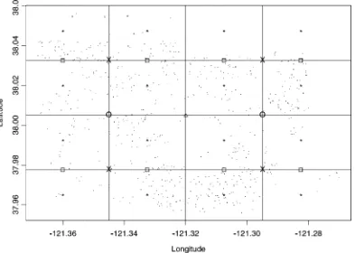
Figure 2. Overlaid Rectangle Showing Knots Resulting From Rectangle Partitioning:1(LD1),±(LD2),£(LD4),¤(LD8),?(LD16).
We have explored the sensitivity to the choice of location for the knots. In particular, for our house price dataset, for a xedL, several sets of knots that cover the region roughly uniformly yielded a BIC that differed by at most 2 from the entries in Table 2 (Sec. 4.2). Furthermore, as expected, the ¯ vector is essentially unchanged (within the accuracy of the simulation-based tting of the models). Hence we have some conrmation of our claim made in Section 1. We need exibility in choosing the number of knots, but givenL, there is robustness to where the knots are. Again, we are not trying to explain the knots.
Evidently, the knots can be developed in many different ways besides our partitioning approach. For instance, they could be attached to an externally determined choice of submarkets. In fact, conceptually, the knots could be random in location and number. Fitting such a model would require a rather sophisti-cated reversible-jump MCMC algorithm (Green 1995) and, in view of the foregoing discussion on matrix computation, might prove computationally infeasible.
4. DATA ANALYSIS
Section 4.1 provides specic details on the priors and the computation. Section 4.2 elaborates on the data analysis.
4.1 Prior and Computational Details
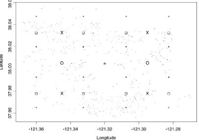
Our illustrative dataset comprises 656 locations in Stockton, California. Of these, 24 sites (6 from each of the 4 quadrants in Fig. 2) were set aside for cross-validation purposes, thereby yielding 632 sites for tting. These latter sites, along with the
L knots.LD1;2;4;8;16/obtained as described in Section 3
are shown in Figure 3. The weight functions®.s;t`/were
com-puted taking° .s;t/Dexp.¡ks¡tk/.
If the covariates are centered and scaled, then a vague prior for¯ would be N.0;cI/forc large. Here, cD104 was set. For computationalexpedience,½ .s¡s0IÁ/Dexp.¡Áks¡s0k/
was chosen. Then the set ofÁ`’s are assumed a priori from
G.:0016; :004/; a gamma distribution with mean :4: This yielded an expected effective range of approximately 7.5 km, slightly less than half of the maximum inter-point distance of 19 km for the whole region and a large variance. All of the posterior summaries are with respect to these units.¿`2and¾`2 were assignedIG.2; :1/priors, that is, a mean of .10 (suitable for our scale) with innite variance.
A hybrid Gibbs sampler was used to t the models. The full conditionaldistributions for the regression parameters were Gaussian. The spatial dispersion parameters,¾`2and¿`2, were updated using a Metroplis–Hastings step with inverse gamma proposals. The spatial range parameters,Á`, do not have stan-dard full conditionals and were updated using a Metropolis step with gamma proposals. Five initially overdispersed paral-lel MCMC chains were run and monitored for convergence us-ing measurements of sample autocorrelations within the chains, plots of the sample traces, and Gelman–Rubin diagnostics (Gelman and Rubin 1992). These diagnostics revealed slower rates of convergence as the number of knots .L/ increased. For example, forLD4;fairly rapid mixing and convergence was obtained within 6,000 iterations, whereas forLD8; the same was seen in approximately 10,000 iterations. ForLD16, 40,000 iterations were required to achieve satisfactory conver-gence.
Figure 3. Sites in Stockton Along With Knots With Varying L.
Banerjee, et al.: Spatial Modeling of House Prices 211
CCC was used as the programming platform. Each itera-tion of the sampler entailed matrix inversion and determinant computations of order 632. To ensure high accuracy for the ma-trix inversions and other linear algebra computations embedded in the iterations, MATLAB CCC libraries were used. These use the highly specialized LAPACK (Linear Algebra Package) to perform the computations (Golub and Van Loan 1996). In our experience, at present the model-tting algorithm proposed in conjunction with (9) can handle sample sizes of perhaps 1,200–1,500 in terms of numerical stability and computational time.
4.2 Data Analysis Details
To explain log selling prices, the following covariates are used in our hedonic specication: square feet of living area (SFLA); a dummy variable denoting whether the lot is large; the age of the property; the number of bedrooms in the home; distance of the home from the Interstate 5 (I-5) highway (a fac-tor anticipated to have an effect on prices of homes in the area); a dummy variable for whether the lot was large or not; a dummy variable for whether the home stands vacant or not; three dummy variables denoting the quarter in which the home went into pending sale (with the rst quarter serving as the baseline). The dataset includes a larger collection of explana-tory variables, but the foregoing choices are those that emerge as signicant under a simple OLS tting.
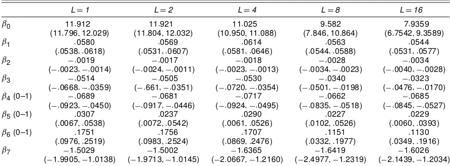
The posterior distributions of the regression parameters have been summarized according to this sequence in Table 1 for the models withLD1;2;4;8, and 16: Among the quarterly dummy variables, only the coefcient of the dummy for the third quarter was signicant (and so is the only quarterly co-efcient shown in the output). All of the remaining covariate coefcients are statistically signicant and behave very simi-larly across the four choices ofL. To clarify, the regression coefcients associated with the covariates are denoted by¯0
for the intercept,¯1 for the coefcient for SFLA, ¯2 for age, ¯3for bedrooms,¯7for the I-5 distance, and¯4; ¯5;and¯6for
the dummy covariates of whether the lot was vacant, whether the property was sold in the third quarter, and whether the lot was large. As expected, the square feet of living area and the size of the lot have a positive impact on the selling price. The
Table 2. Model Comparisons for LD1,2,4,8, and 16
Models ¢(¡2E [ l (µ;Y)|Y]) ¢p 1
NOTE: Here1pdenotes difference in the number of parameters andndenotes the number of observations.
number of bedrooms has a signicant negative impact on the selling price. This may reect the fact that the housing stock in Stockton does not vary greatly in SFLA and buyers may prefer a few large bedrooms to more smaller ones. Homes that were acquired during the third quarter (July–September) were higher priced. Age has the expected negative impact on selling price. Similarly, a vacant home earns a lower price, perhaps because its defects and deciencies are better exposed. Furthermore, va-cant homes may be stigmatized as prospective buyers question the home’s lack of demand. The distance from the important freeway I-5 plays a signicant role; increasing distance reduces selling price. The relationship between log selling price and dis-tance from freeway is not likely to be monotonic; properties very close to the freeway may be devalued due to noise and pollution levels, for instance. However, an examination of the sample of distances in our dataset shows a minimum value of 2.06 km, so we do not think this is an issue in our analysis.
Table 2 presents a model comparison for increasing num-ber of knots using¡2E[l.µIY/jY];where l.µIY/is the log-likelihood, compared with the difference in model dimension multiplied by 12logn;the BIC penalty (Schwarz 1978). Using the BIC, we nd that substantial improvement is achieved by increasing the number of knots from one to two and then from two to four, but a very small gain results from an increase from four to eight. Eight knots are clearly preferred to 16, and so we adopt theLD8 model. As we noted in the previous section, the BIC value was not sensitive to the location of the knots.
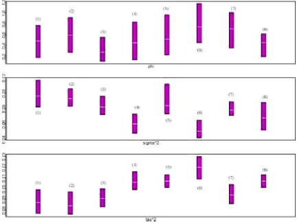
Figure 4 provides posterior summaries for the spatial para-meters forLD8, taking the knots in clockwise order from the upper left in Figure 2. In particular, the spatial variances and error variances in the summary differ signicantly, providing
Table 1. Posterior Summaries for Regression Parameters LD1, 2, 4, 8, and 16
LD1 LD2 LD4 LD8 LD16
Figure 4. Posterior Summary for the Spatial Parameters and the Error Variance Parameter for the Model With LD8. From Figure 2, the order of
the knots is¡8 7 6 51 2 3 4¢in the grid in Figure 2.
justication for the error structure assumed in (2) and (5). With care, these parameters can be given useful interpretations. For example, the variance of the spatial residual attached to a loca-tion near a particular knot will be essentially the variance of the spatial process associated with that knot. So, for example, spa-tial variability is highest near node (1) and lowest near node (6). Also note that across the local models, the spatial variance com-ponent is always at least one-third, and in some cases more than one-half, of the total variance. The spatial story is always con-sequential.
We next consider the conservative rangeeddeveloped in Sec-tion 2 and summarize this acrossLin Table 3. We nd thated in-creases withL (not surprising, considering that we are taking the maximum over more processes), but appears to be reaching an asymptote, further encouraging its interpretation as a range.
Figure 5 shows the 95% prediction intervals for the 24 sites held out from the model tting plotted against the median
pre-Table 3. Estimated Range for the Different Knots
Model ed , km
LD1 6:02
LD2 6:44
LD4 8:93
LD8 10:79
LD16 11:90
NOTE: See text for the denition ofed.
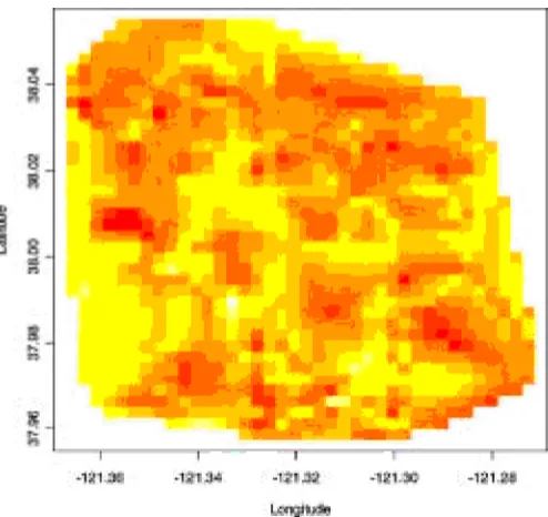
dicted values, along with the observed values indicated by dots, again withLD8. Of these, only one interval does not contain the observed value. Finally, Figure 6 shows a gray-scale plot (nine levels) of the spatial residuals.E.w.s/jY//over the
re-gion. Evidence of a spatial pattern is apparent. For example, properties in the western part of the gure tend to receive a negative spatial adjustment, whereas properties in the southern part tend to receive a positive adjustment.
Figure 5. Prediction Intervals for the Hold-Out Sample Plotted Against Median Predicted Values, With Observed Values Indicated by Dots.
Banerjee, et al.: Spatial Modeling of House Prices 213
Figure 6. Gray-Scale Plot of the Spatial Residuals (posterior mean) Over the Stockton Region, Obtained From the Model With Eight Knots.
5. CONCLUSIONS
In summary, previous literature has used stationarity as-sumptions for spatial process modeling of house prices. Such
isotropicspecication is probably not reasonable, because the spatial association in housing markets likely depends not only on the distance between house transactions, but also where the transactions are located in a city. In this article we have pro-posed a novel, exible and computationally tractable class of nonstationary spatial models and provided an application using data from a sample of single-family house transactions. Specif-ically, we modeled the spatial error across housing prices us-ing a nonstationary process created through locally determined weighted sums of stationary processes. Recognizing that we could not expect local spatial error to explain the residuals en-tirely, we added a distinct pure error process for each local model. We used Bayesian framework for inference purposes and implemented it using Gibbs sampling. The data analysis,
using (log) selling price of house transactions in Stockton, Cal-ifornia, indicated signicance of familiar explanatory variables used in hedonic regressions. Moreover, evidence indicates that there was strong spatial dependence in the error process and that the process was not stationary over the market. Using bi-nary partitioning and the BIC for model selection, the data in-dicated that allowing the number of local stationary processes to increase, up to a maximum of eight, improved the model’s performance. These results encourage the use of nonstationary process models in future spatial modeling of housing markets.
[Received October 2001. Revised April 2003.]
REFERENCES
Agarwal, D. K., Gelfand, A. E., Sirmans, C. F., and Thibodeau, T. G. (2001), “Flexible Spatial Nonstationary Modeling With Application to House Prices,” Technical Report 01-13, University of Connecticut, Department of Statistics.
Cressie, N. A. C. (1993),Statistics for Spatial Data, New York: Wiley. Fuentes, M., and Smith, R. L. (2001), “A New Class of Nonstationary Models,”
technical report, North Carolina State University, Department of Statistics. Gelfand, A. E., Ecker, M. D., Knight, J. R., and Sirmans, C. F. (2004). “The
Dynamics of Location in House Prices,”Journal of Real Estate and Finance Economics, to appear.
Gelfand, A. E., Kim, H.-J., Sirmans, C. F., and Banerjee, S. (2003), “Spa-tial Modeling With Spa“Spa-tially Varying Coefcient Processes,”Journal of the American Statistical Association, 98, 387–396.
Gelfand, A. E., and Smith, A. F. M. (1990), “Sampling-Based Approaches to Computing Marginal Distributions,”Journal of the American Statistical As-sociation, 85, 398–409.
Gelman, A., and Rubin, D. (1992), “Inference From Iterative Simulation Using Multiple Sequences,”Statistical Science, 7, 457–511.
Golub, G., and Van Loan, C. (1996),Matrix Computations, Baltimore, MD: Johns Hopkins University Press.
Green, P. J. (1995), “Reversible-Jump Markov Chain Monte Carlo Computation and Bayesian Model Determination,”Biometrika, 82, 711–732.
Guyon, X. (1982), “Parameter Estimation for a Spatial Process on a
d-Dimensional Lattice,”Biometrika, 69, 95–105.
Haas, T. C. (1995), “Local Prediction of a Spatio-Temporal Process With an Application of Wet Sulfate Deposition,”Journal of the American Statistical Association, 90, 1189–1199.
Higdon, D., Swall, J., and Kern, J. (1999), “Nonstationary Spatial Modeling,” inBayesian Statistics, Vol 6, eds. J. M. Bernardo et al., Oxford, U.K.: Oxford University Press, pp. 761–768.
Schwarz, G. (1978), “Estimating the Dimension of a Model,”The Annals of Statistics, 6, 461–464.
Whittle, P. (1954), “On Stationary Processes in the Plane,”Biometrika, 41, 434–449.