WORKING PAPER #512
INDUSTRIAL RELATIONS SECTION PRINCETON UNIVERSITY
APRIL 2006
New Evidence on Gender Differences in Promotion Rates: An
Empirical Analysis of a Sample of New Hires
Francine D. Blau
*Cornell University and NBER
Jed DeVaro
Cornell University
April 2006
The authors thank Harry Holzer for helpful discussions about the data, the editor and the anonymous referees for helpful comments, and Henri Fraisse, David Rosenblum and Derrill Watson for research assistance.
*For the 2005-2006 academic year, Francine Blau is a Visiting Fellow in the Department of Economics, IR Section at Princeton University (E-mail: [email protected], Phone: (609) 258-6374).
New Evidence on Gender Differences in Promotion Rates: An Empirical Analysis of a Sample of New Hires
Francine D. Blau and Jed DeVaro April 2006
JEL No. J16, J31, J71, M51
Abstract
Using a large sample of establishments drawn from the Multi-City Study of Urban Inequality (MCSUI) employer survey, we study gender differences in promotion rates and in the wage gains attached to promotions. Several unique features of our data distinguish our analysis from the previous literature on this topic. First, we have information on the wage increases attached to promotions, and relatively few studies on gender differences have considered promotions and wage increases together. Second, our data include job-specific worker performance ratings, allowing us to control for performance and ability more precisely than through commonly-used skill indicators such as educational attainment or tenure. Third, in addition to standard information on occupation and industry, we have data on a number of other firm characteristics, enabling us to control for these variables while still relying on a broad, representative sample, as opposed to a single firm or a similarly narrowly-defined population. Our results indicate that women have lower probabilities of promotion and expected promotion than do men but that there is essentially no gender difference in wage growth with or without promotions.
Francine D. Blau
Department of Labor Economics 265 Ives Hall Cornell University Ithaca, NY 14853, U.S.A. Phone: (607) 255-4381 E-mail: [email protected] Jed DeVaro
Department of Labor Economics 268 Ives Hall
Cornell University
Ithaca, NY 14853, U.S.A. Phone: (607) 255-8407 Email: [email protected]
I. INTRODUCTION
Much of the literature on gender differences in the labor market concerns wages. A smaller literature focuses on gender differences in job assignment and, specifically, promotions. Ultimately the two topics are linked, since promotions are typically accompanied by increases in wages. Although an understanding of gender differences in the career experiences of workers in firms requires an empirical analysis that accounts for both promotions and wages, relatively few studies of gender differences in promotions have also considered gender differences in the wage changes attached to promotion. One reason that the omission of wages is problematic is that the concept of a promotion is quite broad. An observation of equal promotion rates between equally-skilled and observationally similar women and men would be misleading if the promotions received by each group differed in quality, with men perhaps receiving the more desirable promotions. We can address this issue to some extent since the wage change attached to a promotion provides some indication of how large a step up the hierarchy a given promotion is, with larger steps usually being accompanied by larger wage increases.1
The empirical literature on gender differences in promotions investigates whether equally qualified men and women with similar observable characteristics have the same chances of receiving a promotion or, more generally, of advancing their careers. Studies in this literature differ in terms of the type of data used; some use data from one or a small number of firms or establishments (with data on many or all of the workers employed), and others use samples of workers (generally resulting in no more than one worker per establishment).
This literature has yielded mixed results. Some studies have found that promotion rates are lower for women than for men with similar observed characteristics (Cabral, Ferber, and Green, 1981; Olson and Becker, 1983; Cannings 1988; Spurr 1990; McCue 1996; Cobb-Clark 2001; Ransom and Oaxaca 2005; Acosta 2005). Others, such as Stewart and Gudykunst (1982), Gerhart and Milkovich (1989), Hersch and Viscusi (1996), Spilerman and Petersen (1999), and Barnett, Baron, and Stuart (2000) have found the reverse. Still other studies have found no significant gender difference in promotion rates. This was the finding in Lewis (1986), Hartmann (1987), Powell and Butterfield (1994), and Paulin and Mellor (1996). Similarly, Giuliano, Levine, and Leonard (2005) found no gender difference in promotion rates, using data from a single, large, U.S. retail employer. And, in a longitudinal study of individual educators in Oregon and New York, Eberts and Stone (1985) found that a gender difference favoring males in the early 1970s diminished and became insignificant by the late 1970s, arguing that equal opportunity
1 We do not mean to suggest that job quality differences are described only by wages. A large number of other factors, for example work-life balance, clearly determine the worker’s perception of the “quality” of a promotion. Nonetheless, the extent of movement up the hierarchy is an important factor in assessing employers’ treatment of observationally similar men and women.
employment enforcement contributed to the decline. Finally, using personnel data for managerial,
administrative and professional occupations within a construction and engineering company, Petersen and Saporta (2004) found no gender differences in promotion after controlling for individual characteristics, though they found higher promotion rates for women in the absence of controls. Their evidence also contradicts the notion of a glass ceiling for women, since promotion rates were higher for men at the low end of the hierarchy and higher for women towards the top of the hierarchy.2
While many previous studies have considered only promotion probabilities and not the wage increases attached to promotions, several have studied both. Olson and Becker (1983) and McCue (1996) found lower promotion rates for women than for men, but comparable wage increases attached to
promotions for the two groups. Gerhart and Milkovich (1989) also found comparable wage increases attached to promotions, though in that study promotion rates were higher for women than for men.
Hersch and Viscusi (1996) and Barnett, Baron, and Stuart (2000) found that women had higher promotion rates but men had higher promotion-associated wage increases. Cobb-Clark (2001) found precisely the opposite pattern: men had higher promotion rates but women had higher wage increases attached to promotions. Finally, using a panel of British households, Booth, Francesconi, and Frank (2003) found that, after controlling for observed and unobserved worker heterogeneity, women are promoted at roughly the same rate as men but receive smaller wage increases from promotion.3
Given the mixed empirical results concerning gender differences in promotions and the limited number of studies that analyze both promotion and compensation, further work in this area remains of interest. Our goal in this paper is to contribute to this literature by analyzing data on promotions and wages for a large sample of recently hired workers spanning many establishments. Our data are of a unique type that has not been used previously in this literature. The sample is from the Multi-City Study of Urban Inequality (MCSUI), a large, cross-sectional survey of employers (establishments) in four metropolitan areas of the United States in the mid-1990s. Many of the survey questions pertain to the establishment’s most recently hired worker, including information on promotions, expected promotions,
2 Similar findings of lower female promotion rates at low levels of the job hierarchy but higher promotion rates higher up in the hierarchy are reported by Tsui and Gutek (1984), Lewis (1986), DiPrete 1989 (chapter 9), Rosenfeld (1992), and Spilerman and Petersen (1999).
3 While these studies used data from the United States, others have investigated gender differences in promotion rates outside the United States. As a whole, the international evidence is somewhat less favorable to women than is the evidence based on US data. Studies finding lower promotion rates for women include Bamberger, Admati-Dvir, and Harel’s (1995) study of two Israeli high-tech companies; Pekkarinen and Vartianinen’s (2004) analysis of panel data on Finnish metalworkers; Sabatier and Carrere’s (2005) analysis of academic researchers in France; and Ranson and Reeves’ (1995) study of computer professionals in a western Canadian city. Wright, Baxter, and Birkelund (1995) compare the U.S., Canada, the U.K., Australia, Sweden, Norway, and Japan, concluding that evidence of lower promotion rates for women is weaker in the U.S. than for the other countries. Also relevant is Winter-Ebmer and Zweimuller’s (1997) finding, based on white-collar workers from the Austrian Microcensus, that females have to meet higher ability standards than males to achieve promotions.
and wages, as well as measures of worker performance, tenure (i.e. the amount of time that has elapsed between the hiring and survey dates), and detailed worker and firm characteristics.
Several features of the data are particularly appealing for an analysis of gender differences in promotions. First, as mentioned, we have information not only on promotions but on the wage increases attached to promotions, allowing us to consider both in the same study. Second, the data include an extensive set of controls for worker and firm characteristics that is paramount in an analysis of gender differences in promotion rates or in any other labor market outcome. Of particular importance on the worker side are direct measures of productivity or job performance. The available measures in this literature are rarely job-specific, and typically the best available proxy is the worker’s educational attainment.4 While we control for education and other worker characteristics, we can also control for performance more completely using numerical job-specific ratings reflecting supervisors’ appraisals of worker performance, as well as the same supervisors’ rating of the performance of “typical workers” in the same job into which the establishment’s most recent worker was hired. This offers an unusual opportunity to control for job-specific worker performance in both an absolute and relative sense. The data sets used in studies in the promotions literature based on broad, representative samples such as ours lack information on worker performance ratings.5
A potential deficiency of the performance ratings, however, is that they might be biased in a way that is correlated with gender. As noted in Blau, Ferber, and Winkler (2006, p. 179), it has been found that identical papers were given higher ratings by students who believed the authors were male instead of female, and similar findings were reported in studies that asked raters to consider the qualifications of applicants for employment.6 Bartol (1999) reviews several field and experimental studies of gender bias in performance appraisals, concluding that findings are contradictory, with some studies finding a bias and others finding no bias. Later in the paper we present some evidence that the gender of the immediate supervisor has no effect on the most recently hired worker’s performance rating in the starting job. While this does not prove that the ratings in our data our unbiased, it does at least cast doubt on certain types of gender-related bias. Further, if there is a bias against women in the performance appraisals, this would serve to lower our estimate of the “unexplained” gender gap in performance—yielding a conservative estimate of this difference (at least with respect to this factor).
4 In addition to educational attainment, Cobb-Clark (2001) controls for AFQT scores in her analysis using the NLSY, though as an overall measure of ability the AFQT score is less directly informative than is a job-specific performance rating.
5 The performance ratings in this survey have been exploited previously in Neumark (1999) in an analysis of gender and racial differentials in starting wages, though that study did not consider promotions or the wage growth arising from promotions. Neumark finds some evidence consistent with employers having worse information about new female than new male employees that may partly explain the lower starting wages paid to women, though he notes that the evidence is not strong from the standpoint of statistical significance.
6 Further information on gender bias in performance ratings can be found in the studies reviewed in Valian (1998) and in Steinpreis, Anders, and Ritzke (1999).
In addition to the worker performance ratings, a further advantage of the MCSUI for our analysis is that it contains a number of firm characteristics that were unavailable for use as controls in earlier promotion studies. For example, the survey includes an indicator for nonprofit status. Our data show that women are more heavily represented in the nonprofit than in the for-profit sector; the fraction working in the for-profit sector is 74 percent for women versus 87 percent for men. Recent empirical work by DeVaro and Samuelson (2005) documents a pronounced difference in promotion rates between for-profit and nonprofit organizations, with promotions less likely in nonprofits. These considerations suggest that nonprofit status should be controlled in analyses of gender differences in promotion rates. To our
knowledge, no prior studies of promotions have had access to data that would allow nonprofit status to be controlled. In addition to nonprofit status, we control for industry, establishment size, number of sites of operation, whether or not the firm is a franchise, and the percentage of workers covered by collective bargaining agreements.
The contribution of an analysis using these data may be illustrated by considering some contrasting studies. McCue (1996) analyzes promotions using the Panel Study of Income Dynamics (PSID), and Booth, Francesconi, and Frank (2003) use the British Household Panel Survey. While both data sets are nationally-representative panels with detailed worker characteristics, they are thin on firm characteristics.7 Furthermore, neither of these data sets contains job-specific measures of worker performance. In contrast, case studies of single firms or small numbers of firms are able to control for firm and job characteristics very precisely, but only by restricting the analysis to one or a small number of firms from which it may be difficult to draw general inferences (e.g. Ransom and Oaxaca 2005 and Giuliano, Levine, and Leonard 2005). Like the studies using broader samples, these single-firm analyses lack individual performance ratings. Our data represent a middle ground that we see as a useful
complement to this literature, particularly given the unique presence of worker performance ratings. We work with a broad, representative sample (though representative of the population of establishments in four major U.S. metropolitan areas rather than a nationally representative sample of workers). At the same time, we are able to control for firm characteristics more precisely than is usually possible with such a broad sample, though inevitably not as precisely as in case studies.
Competing explanations for gender differences in promotion rates may be classified into two broad categories: those that are based on productivity or female preferences for different types of jobs and those that are based on discrimination or broader structural factors. The productivity/preference-based explanations suggest that outcomes (such as promotion rates) may be less favorable for women than men
7 Using data on white men and women from the NLSY, Cobb-Clark (2001) controlled for a limited set of firm characteristics (dummies for two firm-size groups, whether the worker is covered by a collective bargaining agreement, whether the employer has multiple locations, and whether the firm is in the public sector).
due to gender differences in productivity or in job-related preferences (e.g., for authority or demanding positions). Productivity differences could arise due to gender differences in schooling and other pre-market training as well as labor force attachment. Job-related preferences may be influenced by
socialization, among other factors. Gender differences in productivity or job preferences could also arise from the division of labor in the family. For example, Becker (1985) argues that since housework is more effort-intensive than other household activities such as leisure, and since women have historically
performed a greater share of housework than men, married women spend less energy on each hour of market work than men working the same number of hours. This yields lower market wages for women and also induces women to economize on energy expended on market work by seeking less demanding jobs. If this explanation is correct, the presence of job-specific performance ratings offers us a unique opportunity to address productivity-related explanations for gender differences in promotion rates.
Theories of gender discrimination based on personal tastes could take the form of prejudice on the part of employers, customers, or co-workers (Becker 1957). In the case of employer-based prejudice, this would imply that supervisors prefer to manage males rather than females. To the extent that this
preference is stronger for higher-level positions, gender differences in promotion could result. For example, it could be that many managers prefer women in low-level jobs, but not managerial ones (Eagly and Karau 2002).
Theories of statistical discrimination, following early work by Phelps (1972) and Arrow (1973), could also yield gender differences in promotions or wage growth even in the absence of personal prejudice. In such models, employers facing imperfect information about worker productivity rely on certain group characteristics (such as gender) as signals of individual productivity. Lazear and Rosen (1990) offer one such story that gives rise to gender discrimination in promotions. In their model, the employer rationally discriminates against women because gender is correlated with some unobserved factor (such as one’s productivity in nonmarket work, which is assumed to be higher for women than for men) that is relevant to promotions and thereby serves as a signal to the employer.
Either the productivity/preferences or discrimination explanations could lead to promotion differences that are associated with differences in the types of jobs men and women hold. As we have seen, Becker (1985) provides a rationale for women to prefer less demanding jobs. And, models of statistical discrimination suggest that employers may prefer not to hire women for jobs which typically have long promotion ladders.8 Thus, we explicitly investigate the extent to which differences in
8 There is evidence from the sociology literature that longer job ladders tend to be found in jobs and firms that are
predominantly male (Petersen and Saporta, 2004, p. 877), and that the step sizes between levels of the promotional hierarchy are larger for jobs that are predominantly male, implying that promotions yield greater advancement for men than women (Barnett, Baron, and Stuart, 2000).
occupation can explain the residual gender gap in promotion rates. As is well known, the distribution of employment across occupations is quite different for women versus men. If women are more heavily concentrated in occupations with lower promotion rates, this could potentially account for the gender difference in promotions. It is also possible that gender differences in firm characteristics are important for understanding promotion differences. While previous analyses have explored the role of occupation, our data contain information on firm characteristics that have not been available in earlier studies, so it is interesting to see the incremental value of these firm characteristics in explaining the gender gap in promotions. As noted above, one possibility is that women are more heavily represented in the nonprofit sector where promotion rates tend to be lower.
While it is not possible to ascertain whether gender differences in occupation distributions and firm characteristics are due to personal preferences, discrimination, or a combination of the two, it is still of interest to learn the extent to which they constitute the mechanism generating observed gender
differences in promotion rates. Further, the sociology literature emphasizes the importance of sex segregation as a causal mechanism that induces other gender differences in careers (Reskin and Bielby 2005). As noted in Reskin and Bielby (pp. 71-72), “By concentrating men and women in different jobs, segregation exposes them to more or less similar employment practices and reward systems that can, in turn, exacerbate or moderate sex differences in other work outcomes.” More generally, sociologists point out that “structural roles in which individuals find themselves affect their tastes, outlooks, power, social networks, and group loyalties in ways that could not have been anticipated in advance.” (England and Farkas, 1994, p. 345). To some extent then the occupation and industry variables may capture some of these effects. Moreover, it is likely that the unexplained component of the gender gap in our promotion models reflects the impact of such structural factors as well as the impact of discrimination and other unmeasured factors. An unexplained component of the gender promotion gap, even in models such as ours that control for reported job-specific worker productivity, is consistent with Granovetter’s (1994, p. 207) observation that, “Even if productivity were easily gauged, promotions often result from motives or causes not clearly related to it, but easily understandable when relevant social structures and motives are analyzed.”
A potential limitation of our analysis, as with most other analyses of promotions, is that the empirical definition of a promotion is broad, so that a promotion might mean something different for men than for women. The data are not sufficiently rich to rule out this possibility. While we can observe the wage differences arising from promotions, it might be that promotions differ in some other respect (such as prestige) than the compensation attached to jobs. Another limitation is that our analysis is restricted to one worker per establishment, in particular the most recently hired worker. Ideal data would contain
multiple workers per establishment with longer average job tenures than experienced by our sample of recent hires. Furthermore, while we can control for worker characteristics and occupation, we do not observe the hierarchy of jobs in these establishments. For each establishment we observe only a “slice” of the hierarchy, namely the position into which a worker was hired and the position into which s/he has been or could potentially be promoted.
II. DATA: MULTI-CITY STUDY OF URBAN INEQUALITY
We use data from the Multi-City Study of Urban Inequality (MCSUI), a cross-sectional employer telephone survey collected between 1992 and 1995. There are 3510 establishments in the data, and the sampling universe consists of four metropolitan areas: Atlanta, Boston, Detroit, and Los Angeles. The survey respondent was the owner in 14.5% of the cases, the manager or supervisor in 42%, a personnel department official in 31.5%, and someone else in 12%. Screening identified a respondent who actually carried out hiring for the relevant position, and the survey instrument took 30-45 minutes to administer on the telephone, with an overall response rate of 67%. For more information about the data, see Holzer (1996). Our analysis is based on the entire sample, except for seventeen cases we delete in agriculture, forestry, and fishing.
Data were collected in two subsamples and then merged to produce the final release. The first subsample, covering slightly less than two thirds of the cases, was drawn from regional employment directories provided by Survey Sampling, Inc. based on local telephone directories. This subsample (called the SSI sample) was stratified by establishment size (25% 1-19 employees, 50% 20-99 employees, 25% 100 or more employees) and was designed to be self-weighting. It was restricted to employers who had hired a worker within the previous three years for a position that did not require a college degree. The second subsample was drawn from the current or most recent employer reported by respondents in the companion MCSUI household survey, which over-sampled low-income areas and areas with high concentrations of racial minorities. This subsample is not restricted to jobs not requiring a college degree.
Sampling weights adjust for all of these considerations, and we use these weights throughout our study.9 A substantial fraction of survey questions asks about the most recently hired worker, and these questions form the basis for the empirical analysis. The survey asks whether the most recently hired worker has been promoted by the survey date, and the employer’s response to this question is the main dependent variable in the first part of our analysis. We also present results using a measure of expected
9 As stated in the codebook, “[the weights] make use of the link to the MCSUI household file, for those firms that were sampled in this manner, thereby taking account of the household sampling structure and response rates. They also adjust for the fact that the Boston and LA firm samples were incomplete, and the fact that the SSI sample deliberately omits jobs that require college degrees … When the observations in the employer database are weighted by this variable the result should be a representative sample of firms, such as would occur if a random sample of employed people were drawn from each city.” (See Holzer et al. (1998), p. 98.)
promotion as the dependent variable, in particular the employer’s answer to whether or not the most recently hired worker is expected to be promoted within the next five years (regardless of whether a promotion was received by the survey date). The MCSUI data also contain a number of variables
measuring wages and the wage growth attached to promotions. Four variables pertain to the wages of the most recently hired worker: starting wage, current wage at the time of the survey, wage the employee is expected to receive if promoted, and highest wage an employee in this position (the one into which the most recent worker was hired) could attain without a promotion.10 The reported time frames for these
wage questions were either hourly, weekly, monthly, or annually, and we converted all responses to hourly wages measured in 1990 dollars, deflated using the CPI-UX. The second part of our analysis uses three dependent variables that we construct from these four wage questions, as explained in the next section.
III. METHODS
Our analysis consists of two main parts. In the first part, we estimate probit models for the
probability of promotion. In addition, we report results for the probability of expected promotion, though we consider the results regarding received promotions to be of greater interest since they reflect actual, observed outcomes as opposed to subjective expectations about the future. Our goal here is to analyze the extent to which a) reported productivity and b) observable characteristics (i.e. occupation and type of firm) account for any observed gender difference in promotions, when controlling for other measured worker characteristics. We thus report how the gender effect in models of promotion probability changes across a variety of specifications. We begin with a baseline specification that includes as explanatory variables only sex, race, age and age squared, tenure and tenure squared, and educational attainment. We then consider four extensions of the baseline: a) adding only job-specific worker performance ratings, b) adding performance ratings and occupation controls, c) adding performance ratings and firm
characteristics (including industry controls), d) adding performance ratings, occupation controls and firm characteristics. The second part of our analysis concerns wage growth since entering the establishment (focusing on the impact of promotion), potential within-job wage growth in the absence of a promotion, and the expected wage growth attached to expected promotions. Finally, we test one possible source of gender discrimination in promotions by using information on the gender of the most recently hired worker’s immediate supervisor. We explain our methods in more detail in the following subsections.
10 The questions are as follows: “What is the actual starting wage/salary?”; “What is his/her current wage/salary?”; “What is the highest wage or salary that any employee in this position could expect to be paid without promotion?”; “If promoted, what would this employee’s wage or salary be?”
We acknowledge that some of the variables we use as controls in our analyses might be considered endogenous, and in particular might be affected by differences in employers’ treatment of equally
qualified men and women. We have already considered this issue for the performance appraisal variables. Another example would be tenure, the amount of time that has elapsed between the hiring date and the survey date, which could reflect gender differences in involuntary terminations, ceteris paribus, or be influenced by worker responses to perceived differences in treatment at the firm. Also, gender differences in occupations or firm types could be due in part to gender discrimination. As noted above, to the extent such variables are influenced by labor market discrimination, controlling for them could downward bias our estimate of discrimination—the unexplained gender gap in promotions. At the same time the
unexplained gap may in part be due to the impact of unmeasured characteristics related to the productivity or preferences of men and women; an example would be differences between men and women in their preferences for various types of work or for degrees of authority within an organization. In this case, our estimate of discrimination could be biased upward. These considerations suggest caution in interpreting the unexplained gender gap in promotion as an estimate of discrimination.
3.1 Probability of Promotion
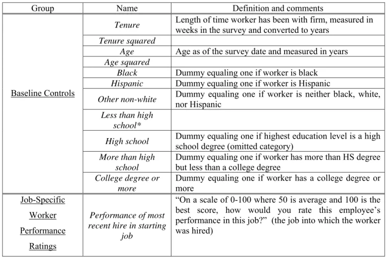
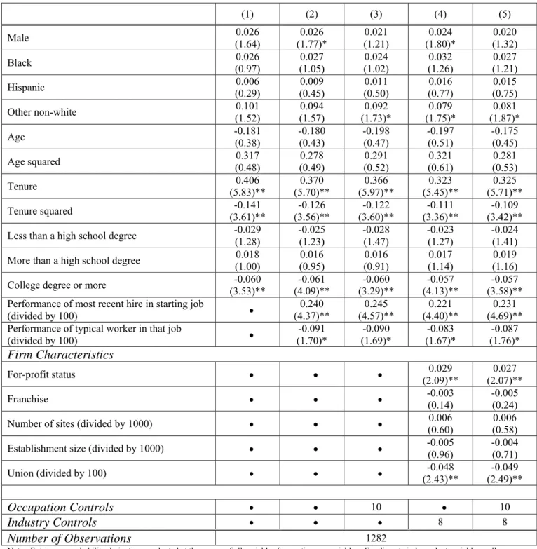
We estimate probit models for the probabilities of promotion (and expected promotion), focusing on how the gender coefficient changes across specifications that include various combinations of the following control variables: age (and age squared), race, tenure (and tenure squared), educational attainment, job-specific performance ratings, occupation and industry controls, establishment size, number of sites of operation, for-profit status, percentage of workers covered by collective bargaining agreement, and whether establishment is a franchise. These variables are defined in Table 1.11
Specification 1 includes only the baseline controls (age, age squared, tenure, tenure squared, race, and educational attainment). As we shall see in the next section, a statistically significant gender gap in promotion rates (favoring men) is found in the baseline model and also unconditionally. A potential explanation for the lower promotion rate of women is that the gender difference reflects productivity differences between men and women. While the baseline specification includes the productivity-proxies like education and tenure generally used in analyses of this kind, an attractive and unique feature of the MCSUI is that it includes job-specific worker performance ratings. Specification 2 adds these
performance ratings to the baseline controls from Specification 1. We then address “location-based”
11 One relevant variable that is not contained in the MCSUI is the worker’s employment experience prior to entering the firm. While we do not observe this variable, we do control for tenure with the firm. More importantly, we control for the worker’s job-specific performance in addition to educational attainment. Since prior work experience would be included in a promotion equation mainly to capture a worker’s skills and ability, it might be argued that it is unnecessary when a direct measure of pre-promotion performance is available.
explanations for gender differences in promotions. To more precisely identify the role of gender differences in employment by occupation versus firm, in Specification 3 we first add only occupation controls along with performance ratings to the baseline model; in Specification 4 we then add only firm characteristics to the baseline and (reported) worker productivity controls. Finally, in Specification 5 we include baseline controls, performance ratings, occupation controls and firm characteristics.
As noted above, we also repeat the analyses described above using “expected promotion” as a dependent variable. We are inclined to put less weight on these results since they relate to expectations regarding promotion, which may or may not be realized. However, they do provide interesting
supplementary information, especially in light of the focus in the data set on recently hired workers.
3.2 Analysis of Wages
We consider three dependent variables pertaining to wages, derived from the four wage variables described in the previous section: wage growth since entering the firm; within-job wage growth attainable in the starting position without a promotion; and expected wage growth attached to expected promotion. We estimate OLS regressions for each of our three dependent variables, using the entire set of controls. Our wage dependent variables are defined as follows:
1. wage growth since entering the firm≡ ln(current wage) – ln(starting wage)
2. within-job wage growth attainable in the starting position without a promotion≡ ln(highest wage
attainable in starting position without a promotion) – ln(starting wage)
3. expected wage growth attached to expected promotion≡ ln(expected wage the worker will receive
if promoted from the starting position) – ln(current wage)
In the regression for the first of these dependent variables, of principal interest is the coefficient on the dummy variable indicating whether the worker has already received a promotion by the survey date. This parameter provides information about the average additional wage growth associated with having been promoted as compared with not having been promoted. A potential problem with this interpretation is that, obviously, individuals who have been promoted may differ from those with similar measured characteristics who have not been promoted. If they are, for example, a positively selected group, they may have earned more than otherwise similar individual even if they had not received a promotion. Unfortunately, we lack a variable that could identify a simultaneous model of promotions and wage determination. While we acknowledge that it may not be possible to give a causal interpretation to the coefficient on a promotion indicator in an OLS wage regression, the estimated return to promotion does
yield interesting descriptive information, which is at least suggestive of the extent of gender differences in returns to promotion.12
The second of these dependent variables, potential within-job wage growth, is interesting because the consequences of not getting promoted may differ between men and women. For example, one possibility is that higher promotion rates for men are counterbalanced by higher rates of anticipated within-job wage growth for women. It is therefore important to consider expected wage growth in the absence of promotions in addition to the wage growth attached to received and expected promotions. The wording of the question pertaining to the “highest wage attainable without a promotion” refers to “any employee in this position” rather than to the specific individual. On the one hand, a positive feature of this wording is that this information is available for all workers, whether or not they have been promoted. On the other hand, a potential measurement problem is that it is not necessarily the case that the focal worker (i.e., the most recent hire) would have achieved the indicated wage. So, for example, suppose the most recent hire is female and that the establishment engages in wage discrimination against women. The highest wage that this worker could receive in her starting position is unobserved in the data, and the answer the respondent reports as the highest wage attainable in that position could pertain to the
maximum a male could expect to receive in the same position. In light of this issue, the results based on this dependent variable should be interpreted cautiously. If it is true that the “highest wage attainable” in the position is more likely to be defined by what a male could attain than by what a female could attain, this would cause us to underestimate gender differences in compensation.
We define the third dependent variable, expected wage increase attached to expected promotion, only for those workers for whom a promotion is expected, estimating the model only for these workers.13 For this regression, we also report a specification that includes the promotion dummy on the right-hand-side as a control.
A theoretical model based on “sticky floors” was proposed in recent work by Booth, Francesconi, and Frank (2003). The term “sticky floors” refers to the situation in which women are promoted as often as men but receive lower wage gains attached to promotion. In firms with formal wage scales, women remain stuck to the lower wage levels on the wage scale of their new, higher job grade following
12 Another issue is that the data do not indicate how many promotions the worker has received since being hired. So if some workers have been promoted more than once since the starting date, the estimated promotion effect will overestimate the average wage increase associated with a single promotion. However, since the sample is one of recent hires, only nine percent of whom have been promoted by the survey date, we think this is unlikely to be a serious problem; few of these workers will have had time to be promoted more than once since the hiring date.
13 If we also include those workers for which a future promotion was not expected but an actual promotion had already been received -- defining the “wage change attached to promotion” as the log-difference between the current (post-promotion) wage and the starting (pre-promotion) wage – we add only 8 observations to the male regression and 9 observations to the female regression, and the results are virtually unchanged.
promotion. This can arise either due to women’s inferior market alternatives or to less favorable responses on the part of their employer to bids for their services from outside employers. The authors find evidence consistent with their model’s main predictions, using panel data spanning the years 1991-1995 from the British Household Panel Survey. Since we also address wage increases attached to promotion in our study, we will also evaluate the “sticky floors” hypothesis on our sample of promotion decisions for recent hires in establishments in four American metropolitan areas.
3.3 Gender Discrimination Arising from Employer Prejudice
In both the promotion analysis and the wage analysis, the set of control variables is extensive and includes job-specific performance ratings to capture (reported) worker productivity in a more detailed way than is possible with the usual controls for educational attainment. This raises the question of how gender differences in promotions or wage growth should be interpreted. One conventional interpretation is that the residual gender gap is due to discrimination. However, as noted above, in this as in other similar analyses, such differences in promotions (or wage growth) could reflect unobserved differences between men and women that are correlated with promotions. While our data do not allow us to decompose the unexplained promotion difference into the part due to discrimination and the part due to unobserved heterogeneity, some indirect evidence allows us to speculate about the nature of the gender discrimination that might be present in promotion decisions.
The MCSUI data contain information allowing us to investigate the possibility of gender discrimination based on personal prejudice on the part of the employer. We observe the gender of the most recently hired worker’s immediate supervisor, who likely exerts strong influence on this worker’s promotion prospects if not determining them entirely. We define the following dummy variable:
Male Supervisor: dummy equaling one if the most recently hired worker’s immediate supervisor
in the starting job is male, and zero otherwise
We include this variable and its interaction with the Male dummy variable in the probit models for
promotion and expected promotion. Taste-based discrimination against women (such that male supervisors tend to underpromote women relative to men) would imply a negative coefficient on Male Supervisor, and a positive coefficient on (Male × Male Supervisor).14 In our wage models (which are
14 Note that the key expectation would be a positive coefficient on (
Male × Male Supervisor) since the main effect of Male Supervisor could be influenced by the propensity of male versus female supervisors to promote in general. So for example, if
estimated separately for men and women) we include the Male Supervisor dummy as a control and report
its coefficient. Widespread discrimination based on personal prejudice on the part of the employer should imply a negative and statistically significant coefficient when this dummy is included in the equations for women.15
Of course, the foregoing assumes that female supervisors do not discriminate against their female subordinates in promotion decisions and wage decisions. A theory that is at odds with this assumption is the “queen bee syndrome”, as defined by Staines, Tavris, and Jayaratne (1973). According to this
syndrome, women who are individually successful in male-dominated environments and attain positions of high status are more likely to endorse gender stereotypes. That is, they tend to view the women they supervise as competitors and possess negative attitudes towards them, making them more likely to discriminate against these female subordinates. However, the empirical analysis in (Terborg et al. 1977) suggests that women with higher education levels hold the most favorable attitudes toward female managers. If one’s level in a promotional hierarchy is an increasing function of education, then these results are in conflict with the queen bee syndrome. From the perspective of our analysis, if females as well as males discriminate against females, then women’s adverse promotion or wage outcomes may not be associated with supervisor gender, but this finding would not necessarily imply that there was no employer discrimination against women. Moreover, it is worth emphasizing that this exercise is only pertinent to taste-based theories of discrimination in which the prejudicial views are held by the employer, and not to prejudice by customers or co-workers or due to statistical discrimination.
IV. EMPIRICAL RESULTS
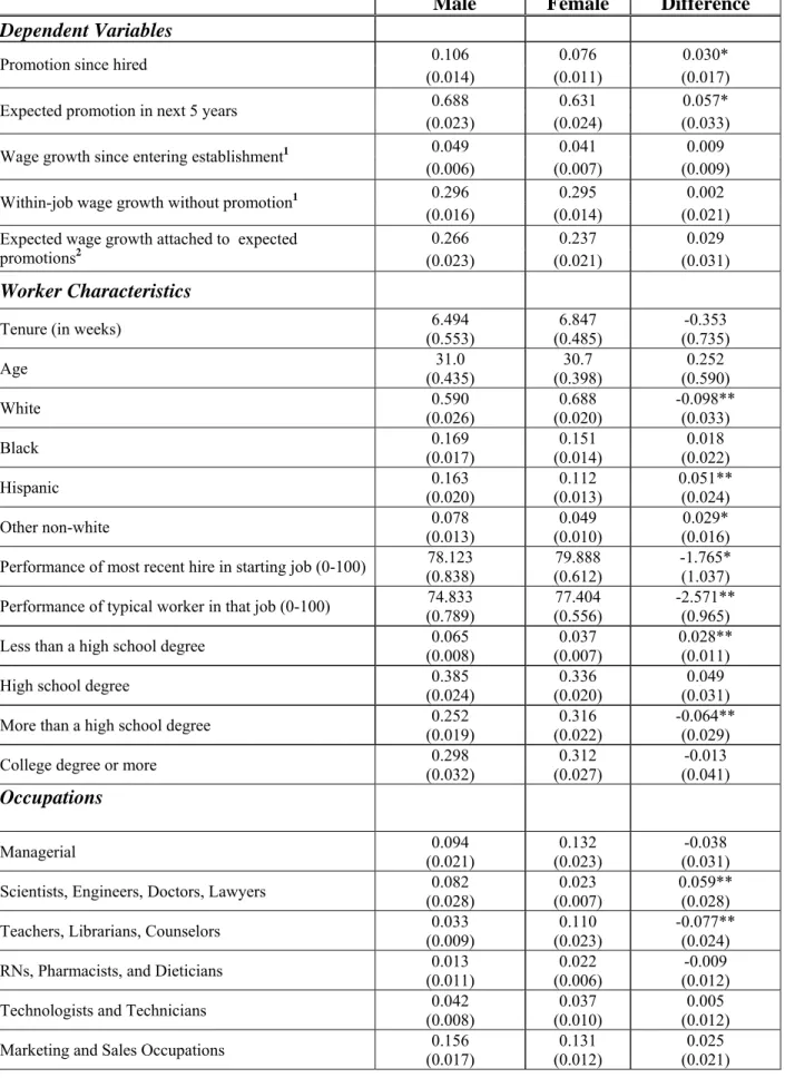
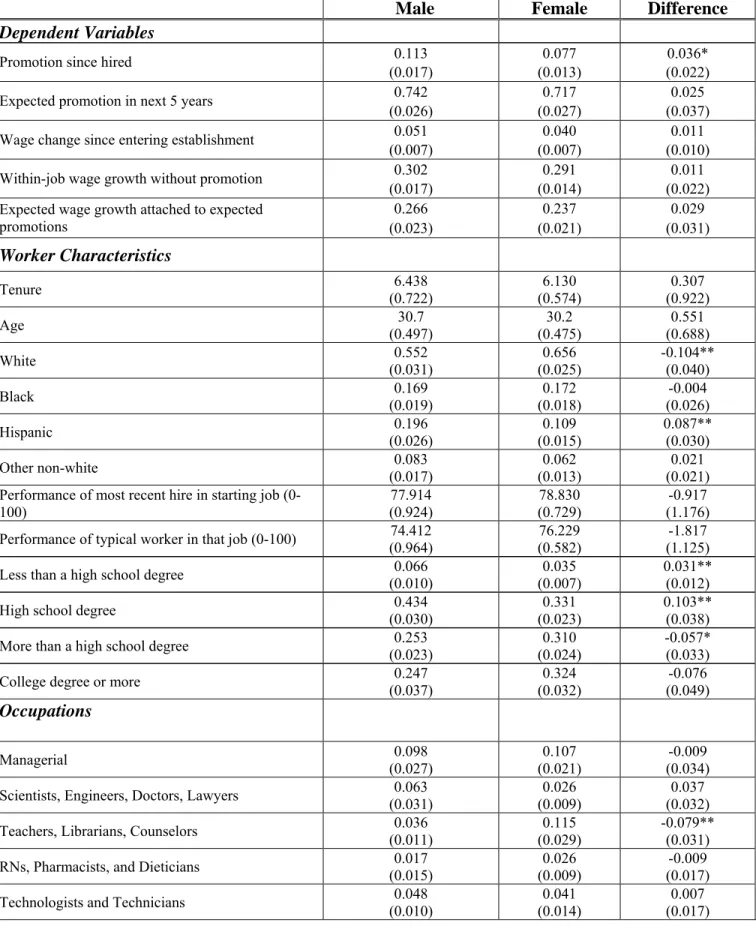
Summary statistics for all variables in our analysis are displayed in Table 2 for the subsamples of males and females. The fraction of males in the sample is 48 percent. This is significantly lower than the fraction of males in the working population. But recall that the survey is a random sample of recent hires (one per establishment), not a random sample of workers. Given this sampling scheme, if we consider the gender of the most recently hired worker it is not surprising that this worker is roughly equally likely to be a male as a female. The fact that the fraction of female workers is higher in our sample than in the
working population does not present problems for our analysis, since our goal in this paper is to compare differences in employer behavior towards women and men in a sample of new hires spanning many establishments.
and females might have higher promotion rates when they have a male supervisor. However, in the presence of gender
discrimination, the interaction of male and male supervisor is expected to be positive.
15 We again note that, considering the preceding footnote, the stronger prediction would be that the coefficient on male supervisor be larger in the male than in the female equations.
The first row of Table 2 reveals that, unconditionally, promotion rates are higher for men than for women. The fraction of received promotions is relatively small for both sexes (10.6 percent for men and 7.6 percent for women) because in a sample of recent hires most workers will not have been with the firm long enough to have received a promotion. Nonetheless, the gender difference of 3.0 percentage points is large in relative magnitude (39.5 percent) and statistically significant. As seen in the second row, rates of expected promotion are also higher for men than for women, and the fraction of expected promotions is relatively high for both sexes (68.8 percent for men and 63.1 percent for women); recall that the relevant question concerns the expectation of promotion within the relatively long window of the “next five years.” And, the gender difference of 5.7 percentage points, while also statistically significant, is smaller in relative magnitude (9.0 percent). With respect to wage growth since starting the job, potential for within-job wage growth in the absence of promotion, and the expected wage growth attached to expected promotions, the means are slightly higher for men, but the differences are not statistically significant.16
The male and female subsamples are similar in average age and tenure with the firm. Men are more likely to have less than a high school degree and women are more likely to have some college; the fraction with a college degree or more is similar for men and women. With regard to race and ethnicity, the female workers are more likely than the males to be white and less likely to be Hispanic or “other nonwhite”. The average performance of the most recently hired worker in the starting position is somewhat higher for women than for men, as is the average performance of the typical worker in that position. A potential explanation for the latter result is that establishments for which the most recent hire is female may be more likely to hire women, so that the “typical worker” in the relevant position is likely also to be female. As suggested in our sample and noted earlier in Neumark (1999), females appear to have higher job performance on average than do males.
Focusing on the gender differences in means that are statistically significant, men are more highly represented than women in the following occupational groups: “Scientists, Engineers, Doctors, and Lawyers” (by 6 percentage points), “Craft, Construction, and Transportation” (by 16 percentage points), “Production Workers and Laborers” (by 11.5 percentage points), and women are more highly represented than men in “Teachers, Librarians, Counselors” (by 8 percentage points) and in “Administrative Support Occupations, Including Clerical” (by 26 percentage points). Across industries, men are more highly represented in mining and construction (by 2 percentage points) and manufacturing (by 13 percentage points), while women are more highly represented in finance (by 5 percentage points) and services (by 19
16 Wage levels, as opposed to wage growth, are higher for men than for women. The average hourly starting wage was $9.87 for men in our main estimation sample and $9.31 for women, though the difference is statistically insignificant (t = 0.82). The average hourly current wage (as of the survey date) was $10.42 for men and $9.56 for women, with the difference in means statistically significant only at the 10 percent level on a one-tailed test (t = 1.31). All wages are deflated to 1990 dollars using the CPI-UX.
percentage points). The only other firm characteristic with a noteworthy gender difference is for-profit status (86.9% for men and 73.7% for women).
4.1 Probability of Promotion
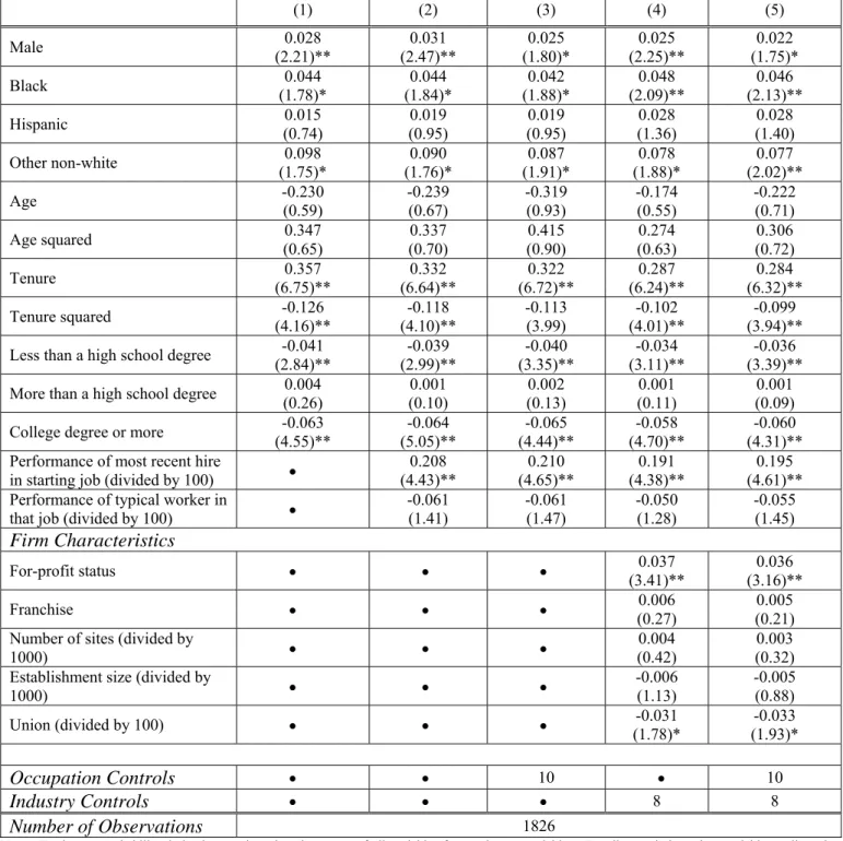
We next ask whether the gender difference in promotion rates observed in the first row of Table 2 persists after controlling for worker and firm characteristics, as well as how it changes across different specifications of control variables. As seen in our baseline specification of the promotion probit (Column 1 of Table 3), the difference in the predicted probability of promotion between men and women
(evaluating the other covariates at their means) is 2.8 percentage points, virtually the same as the
unconditional gender difference in promotion rates in the first row of Table 2.17 As seen in Column 2 of Table 3, in the presence of controls for job-specific worker performance ratings the gender effect actually increases slightly to 3.1 percentage points, remaining significant at the five percent level. This result casts some doubt on the hypothesis that women’s lower promotion rates in the baseline model is due to lower reported female productivity.
Another potential explanation for the gender difference in promotions is differences in the types of jobs held by women versus men. If women are more heavily concentrated in occupations with lower promotion rates, this could potentially account for the gender differences in promotions. In this event, adding controls for occupation would reduce the magnitude of the gender effect. As seen in Column 3, the gender effect decreases only modestly to 2.5 percentage points and remains statistically significant at the ten percent level. A hypothesis test that the coefficient of Male is the same between columns 2 and 3 cannot be rejected (t = 0.71).
It is also possible that the gender differences pertain to firm characteristics; we have particularly noted for-profit status as a potentially important gender difference in employment by firm. Comparing columns 2 and 4, we see that the gender effect decreases to 2.5 percentage points in the presence of for-profit status and other firm characteristics, and it remains significant at the five percent level. However, a hypothesis test that the coefficient of Male is the same between columns 2 and 4 cannot be rejected (t = 0.71). Finally, if both occupation controls and firm characteristics are included, a comparison of columns 2 and 5 reveals that the gender effect decreases to 2.2 percentage points, achieving significance at the ten percent level. However, a test of the hypothesis that the Male coefficient is the same between columns 2
17 As in the recent papers by Booth, Francesconi, and Frank (2003) and Giuliano, Levine, and Leonard (2005), our analysis pools men and women in a single equation. We have also considered separate promotion equations for men and women, and these results are available upon request. The gender effects of interest that are found by estimating separate promotion models for men and women are qualitatively similar to those we present here.
and 5 cannot be rejected (t = 0.87). In summary, neither the job-specific performance ratings nor the occupation controls and firm characteristics change the estimated gender gap in promotions very much.
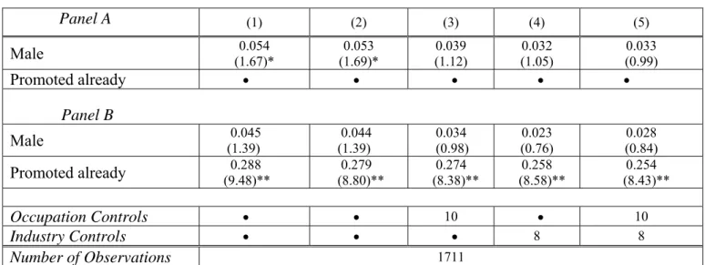
We also repeated the analysis using “expected promotion” as a dependent variable, though we note that employer views on expected promotion may reflect expectations about differentials in quits and family leave by sex, particularly in this relatively young sample of recent hires. Results for probability of expected promotion are displayed in Table 4. Panel A of Table 4 reports results from models that include the same configurations of explanatory variables as in Table 3. Panel B is the same, except that it also includes a control for whether the most recent hire had already been promoted by the survey date, since whether or not a future promotion is anticipated may plausibly be affected by whether or not one has already been received. We note, however, that if the gender difference in promotions received as of the survey date reflects discrimination, this is held constant in our model of expected promotion that includes received promotions as a control. In any case, the pattern of results in both panels of Table 4 is similar. The probability of expected promotion is roughly four to five percentage points higher for males than for females, in both the baseline specification and the specification that adds worker performance ratings. In Panel A, these results are statistically significant at the ten percent level, and that is also the case in Panel B if a one-tailed test is used as the criterion for significance. While the absolute gender difference is larger than was the case for actual promotions, the ceteris paribus gender difference is considerably smaller relative to the mean. Moreover, unlike our results for actual promotion, in both panels the
inclusion of either occupation controls or firm characteristics shrinks the gender gap in expected promotions and renders it statistically insignificant. Thus, there seems to be more support for location-based explanations for the gender gap in expected promotions than there was in Table 3 for received promotions.18
Across all specifications in Table 4 the coefficient on the received promotion dummy was positive, statistically significant, and large in magnitude. Other things equal, workers who have already received a promotion by the survey date are more likely (by more than 25 percentage points) to have a promotion expected within the next five years. One potential explanation for this is unmeasured worker characteristics such as ability. We think this explanation is unlikely, however, since the magnitude of the effect remains virtually unchanged when worker performance ratings are added to the baseline
specification. If unobserved worker ability is the driving force, and if the job-specific performance ratings at least partially capture worker ability (which seems a reasonable assumption), then the
magnitude of the coefficient on received promotion should clearly decrease when performance controls
18 As in our analysis of received promotions, we also considered separate equations for men and women in the analysis of expected promotions. Our results on the gender effect of interest were qualitatively similar to those we report here.
are added to the model. An alternative explanation for the finding is that there are unobserved firm and job characteristics, such as detailed industry and occupation, that are correlated with promotions. This too, however, seems unlikely. If the promotion coefficient is picking up unobserved detailed industry and occupation variables, then the magnitude of the promotion coefficient should change when our (coarser) occupation and industry controls are included in the specification, since the detailed categories are likely correlated with their coarser aggregates. In fact, the promotion coefficient is relatively insensitive to the inclusion of occupation controls or firm characteristics. Another potential explanation is the commonly-observed workplace practice of offering promotion “fast tracks.” Fast tracks in promotions mean that workers who have been promoted quickly in the past are likely to be promoted quickly again in the future, even controlling for performance. A number of theoretical models yield this prediction (Bernhardt 1995; Prendergast 1992; Meyer 1991).19
4.2 Analysis of Wages
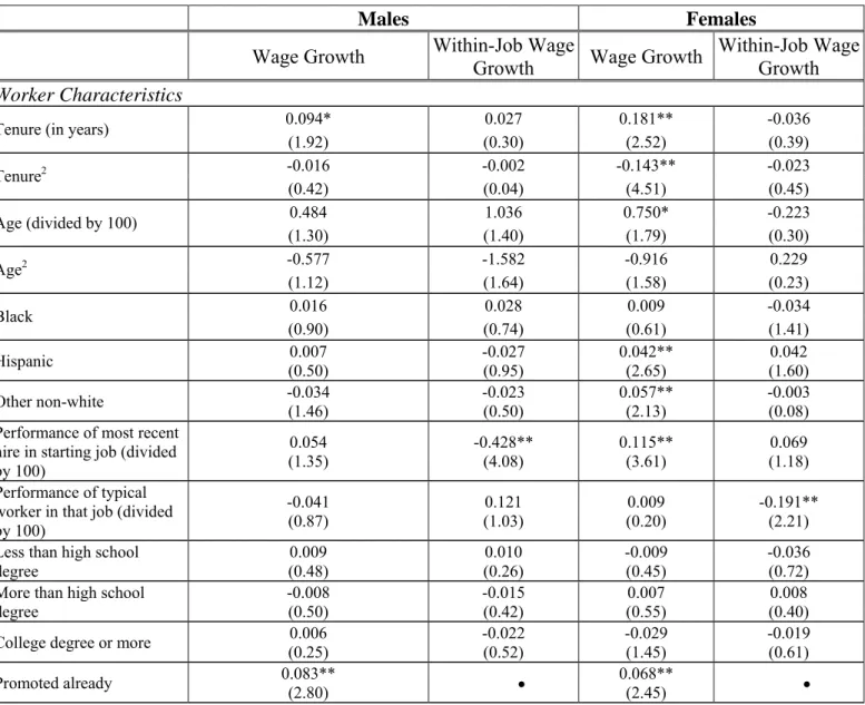
Columns 1 and 3 of Table 5 display regression results for the dependent variable “wage growth since entering the establishment.”20 Of principal interest is the coefficient on the promotion dummy variable which suggests that, for both women and men, promotions are associated with average wage increases of about seven to eight percent over the starting wage. The Oaxaca (1973) decompositions in the last row of the table indicate that, regardless of whether the male or female weights are used, there is
19 Another interpretation of the positive coefficient on received promotions is that some establishments are experiencing and expecting growth, so promotion rates will be higher in the past and future. To address this, following DeVaro and Samuelson (2005) we construct a measure of the monthly net change in employment for each establishment. The survey asks the
respondent employer what the net change in the establishment’s total number of employees has been since the start of 1992 (or 1993 for a small subset of observations collected by Kirschenman, Moss, and Tilly (KMT) towards the end of the data
collection effort). Using the interview dates (which range from 6/8/1992 to 3/15/1995), for each observation we compute a variable called “months” measuring the number of months that elapsed between the start of 1992 (or 1993 for the KMT observations) and the survey date, using the day of the month to compute fractional months. Since no interview dates were recorded for the KMT observations, for these we set the survey dates to 3/15/1995, the midpoint of the data collection period for these observations. We then define a monthly net change measure as follows:
Net change = (net change since start of 1992) / (establishment size × months)
When this variable is included as a control to the specifications in Table 4, Panel B, the coefficient on received promotions remains positive and statistically significant in all cases and roughly the same in magnitude. This suggests that the positive relationship between received and expected promotions reflects more than just differences in monthly employment growth rates across establishments.
20 The subsamples in this table are smaller than in the promotion analysis of Table 3, due to missing values in the wage variables. Since the primary goal in this paper is to study gender differences in promotion rates, our preferred set of estimates for promotion probabilities are those reported in Table 3 that use all available observations. However, we also checked to see how our main results would change when the models for promotions were estimated on the smaller subsample from the wage analysis. Results are in Appendix Table A2 (descriptive statistics for this smaller subsample are also reported in Appendix Table A1). Given the reduction in the sample size, the gender effects in Table A2 are estimated with lower precision than in Table 3 and sometimes fail to achieve statistical significance at conventional levels. Nonetheless, the Z-statistics always exceed one. Furthermore, the magnitude of the effect ranges from 2.0 to 2.6 percentage points, which closely matches what we found in Table 3.
little difference between women and men in the wage growth experienced since the starting date.21 An interesting result is that worker and firm characteristics matter for female wage growth but not male wage growth. Focusing on results that achieve statistical significant at the ten percent level, female wage growth is negatively associated with both tenure and the percentage of employees covered by a collective bargaining agreement, and positively associated with Hispanic or other non-white status (relative to whites), job-specific performance, and number of sites of operation. Of these factors, only tenure has a statistically significant association (positive in sign) with male wage growth.22
Columns 2 and 4 of Table 5 display regression results for the dependent variable “within-job wage growth without a promotion.” The Oaxaca decompositions in the last row of the table indicate that when male weights are used the difference favors women whereas when the female weights are used the
difference favors men. These relatively small differences on the order of one percentage point parallel the unconditional results from Table 2, which revealed essentially no gender difference in within-job wage growth. While the conditional results in columns 2 and 4 of Table 5 also suggest no substantial gender difference, recall that they may underestimate the gap favoring men, since, as explained above, the dependent variable is based on a question about the highest wage that any employee in this position
[meaning the starting position of the most recent hire] could expect to attain without a promotion. The results in columns 2 and 4 of Table 5 should therefore be interpreted with caution.
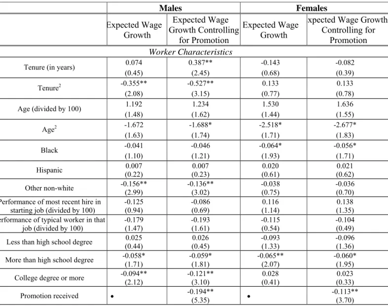
Table 6 displays the regression results for the dependent variable “expected wage growth attached to expected promotions” that we estimate only on the subsample of workers for whom a promotion is expected.23 Columns 2 and 4 are the same as columns 1 and 3, respectively, except for the inclusion of a dummy indicating whether a promotion has already been received. The main result is that when the promotion dummy is excluded from the regression, we find a small difference favoring women when the male weights are used and a small difference favoring men when the female weights are used, though in both cases these differences are well below one percentage point. When the regression controls for received promotions, the Oaxaca decompositions using either set of weights reveal differences favoring men (0.3 percentage points using male weights and 1.7 percentage points using female weights). Relative to the mean wage change attached to expected promotions, which is 25 percent, these gender differences range from a 0.5 percent change favoring women (when the promotion dummy is excluded and male
21 As noted above, wage levels, as opposed to wage growth, are higher for men than for women, although not always significantly so.
22 Another approach for investigating gender differences in the wage growth attached to promotion is to focus only on the subsample of promoted workers. Though the sample size is small (N = 149), a regression of wage growth on a gender dummy and the full set of controls for the sample of promoted workers yields an estimated coefficient of
-0.044 on the Male dummy, with a standard error of (0.044).
23 We could not take an analogous approach for received promotions (that is, estimating a model of the wage increase in the subsample of promoted workers) since the subsample of received promotions is too small.
weights are used) to a 6.7 percent change favoring men (controlling for received promotions and using female weights). The midpoint of this range is near the unconditional difference in means of 2.9 percentage points found in Table 2. An interesting point is that establishment size is statistically
significant in these regressions but in none of our earlier models. Given that most labor market outcomes vary by size it is interesting that the probabilities of promotion and expected promotion, as well as wage growth since entering the firm, and within-job wage growth without a promotion appear not to be
associated with establishment size. For both men and women, establishment size is negatively associated with the expected wage growth attached to expected promotions.
To summarize the wage analysis, our main finding is that promotions yield roughly similar wage increases for men and women. We interpret this as descriptively showing that the returns (in terms of higher wages) to promotion are the same or similar for women versus men. A causal interpretation cannot be attached to the promotion coefficient, since, as discussed above, a selection effect might be operating whereby unobserved characteristics (for example, unobserved components of worker ability) determine both promotions and the wage increases attached to expected promotions. The selection bias is likely to cause us to understate the extent to which wage increases attached to promotion are higher for men than women. For example, if discrimination against women means that men are promoted farther down in the skill distribution than women, then promoted women are of higher average quality than promoted men. Thus, our finding of no observed gender difference in wage returns from promotion would actually imply a lower return for women than men of equal quality. Similarly, we find little consistent evidence of
gender differences in the expected wage change attached to expected promotions; our results suggest no meaningful difference if male weights are used and a modest difference favoring men if female weights are used.
The fact that the wage growth accompany promotion is not smaller for women than men is not consistent with the “sticky floors” model proposed by Booth, Francesconi, and Frank (2003) and tested using data from the British Household Panel Survey. Whereas they found roughly the same promotion rates for men and women but lower wage increases from promotion for women, we find that women are promoted less frequently than men but that the wage increases attached to promotion are roughly
comparable for both sexes (as did Olson and Becker 1983 and McCue 1996).
A Test of the Consistency of the Observed Gender Differences With Employer Discrimination
To address taste-based models of gender discrimination we now turn our attention to the gender of the most recent hire’s immediate supervisor in the starting position, recalling that Male Supervisor is a
position was male, and zero otherwise. There is a large gender difference in the likelihood of having a male supervisor. Seventy-eight percent of recently-hired men have a male supervisor versus only forty-one percent of women.24 This large, unconditional gender difference in the likelihood of having a male supervisor likely reflects underlying differences in representation of women across sectors.
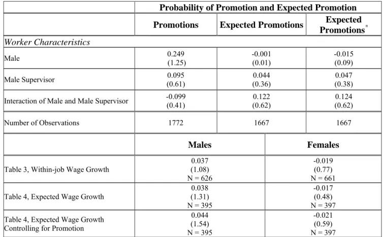
Table 7 displays the results from incorporating supervisor’s gender into our models of promotion, expected promotion, and wage growth. In each case we present results from our most fully specified model, including, in addition to the baseline controls, performance measures, occupational dummies and firm characteristics. In the models for the probabilities of promotion and expected promotion, taste-based discrimination (whereby male supervisors tend to underpromote women relative to men) would imply a negative coefficient on Male Supervisor, and a positive coefficient on the interaction of Male and Male Supervisor. The results do not support this; whether the dependent variable is received promotions or
expected promotions, the coefficients of interest frequently have the wrong sign and in all cases are far from statistically significant at conventional levels. In the lower panel of Table 7 we report the
coefficients on Male Supervisor in the various wage growth models, which are estimated separately for
men and women. In each model, the coefficient on Male Supervisor is statistically insignificant, casting
doubt on the notion of gender discrimination based on male supervisor prejudice, although an alternative interpretation is that female supervisors also discriminate against their female subordinates in determining promotions and wages.
Giuliano, Levine, and Leonard (2005) discuss an interpretation of these coefficients in the context of the theory of social roles (Eagly 1987). Social role theory argues that certain social roles (which generally coincide with social status norms) are expected of individuals by society based on the particular groups to which they belong. When workplace relationships deviate from the expected social roles (for example, when a female supervises a male), both supervisors and workers can become uncomfortable (Kanter 1977, Eagly 1987, as cited in Giuliano, Levine, and Leonard 2005).25 Though in the present context the relevant “role breaking” relationship would be a female supervising a male, Giuliano, Levine
24 Using data from the NLSY for workers aged 17 to 25, Rothstein (1997) found that in 1982 the fraction of men with a male supervisor was 0.91 and the fraction of women with a male supervisor was 0.53. The decline for both women and men in the likelihood of having a male supervisor is consistent with the increasing participation rate for women during the 1980s. Future users of this variable in the MCSUI employer survey obtained from the ICPSR data archive should make note of a labeling error in the raw data. The variable containing the supervisor’s gender is called “c35” in the codebook and equals 1 if the supervisor is female and 5 if male. The text labels attached to these observations are reversed, however, with “male” being assigned to females and “female” assigned to males. To avoid an error, the text labels should be ignored and only the
underlying numerical codes (1 = female, 5 = male) should be used. We are grateful to Harry Holzer for his help in identifying this problem.
25 As noted in Reskin and Bielby 2005 (p. 78), “Qualitative research suggests the possibility that men in predominantly female jobs advance more quickly than their female co-workers because their supervisors are uncomfortable with men doing
customarily female jobs (Williams, 1992). However, the advancement gap between the sexes stems in part from sex composition of jobs, according to quantitative analyses showing that men in predominantly female jobs are promoted more slowly than their counterparts in mixed-sex or predominantly male jobs (Budig, 2002).”
and Leonard 2005 consider other possible role breaking relationships, such as young supervisors of older workers or non-white supervisors of white workers.
The discomfort experienced by both parties to a role breaking relationship can lead to two different types of outcomes. On the one hand, given that males belong to traditionally higher-status groups, a male worker supervised by a female is more likely to resent and disrespect the female manager than he would a male manager, and this might result in less desirable outcomes for the male worker (e.g. lower rates of promotion or expected promotion, or lower wage growth attached to promotions). In the context of our estimated models, this would imply that the sum of the Male Supervisor coefficient and the Male × Male Supervisor coefficient was negative (so that male workers fare worse under a female
supervisor than under a male supervisor). On the other hand, traditionally lower-status workers who find themselves in supervisory roles might defer to traditionally higher-status workers, refraining from
exercising authority over them. This might lead to better outcomes for males supervised by females (such as higher rates of promotion or expected promotion, and higher wage increases attached to promotion). In the context of our estimated models, this would imply that the sum of the coefficients on Male and Male × Male Supervisor is positive (so that male workers fare better under a female supervisor than under a male
supervisor). Since either or both of these possibilities could be present in the data and the reactions to role breaking relationships could differ across establishments, social role theory does not offer a clear
prediction on the signs of our coefficients in Table 7.
A potential concern discussed above is that a discriminating employer might give female workers lower performance ratings than similar male workers would receive. This could mask gender
discrimination in promotions because men and women with equal performance reported by the supervisor received the same treatment (with respect to promotion and wages), while in fact women would have to be more productive than men to receive the same performance rating. To investigate this possibility, we checked for a relationship between the subjective performance rating and the gender of the immediate supervisor. If discrimination in performance evaluations were widespread in our sample, we would expect to see that women with male supervisors would have lower scores, on average, than women with female supervisors. In fact this is not the case.26 However, we note that, as mentioned earlier, this result does not preclude the possibility of gender discrimination on the part of both male and female supervisors,
26 A regression of the performance rating on Male, Male supervisor, and Male × Male supervisor (as well as the controls for worker characteristics, occupation, industry, and firm characteristics) yields a Male coefficient of -0.007 (t = 0.45), a Male supervisor coefficient of 0.009 (t = 0.64), and a Male × Male supervisor coefficient of -0.001 (t = 0.04). Since these estimates are far from statistically significant, this provides some evidence that the performance rating likely means the same thing for women as for men, at least under the assumption that male supervisors potentially discriminate against women and female supervisors do not.