Mathematical Programming Models For Portofolio Selections.

Supian SUDRADJAT

Referenţi ştiinţifici: Prof. univ. dr. Vasile PREDA Prof. univ. dr. Ion V DUVA

@ editura

universit

ţ

ii din bucure

ş

ti

Ş

os. Panduri, 90-92, Bucure

ş

ti-050663;Telefon/Fax: 410.23.84

E-mail:editura_unibuc@yahoo.com

Internet:www.editura.unibuc.ro

Descrierea CIP a Bibliotecii Na

ţ

ionae a Romaniei

SUDRADJAT, SUPIAN

Mathematical programming models for portfolio selection /

Supian Sudradjat – Bucure

ş

ti: Editura Universitt

ţ

ii din

Bucure

ş

ti, 2007

ISBN 978-973-737-351-9

This work would not have been possible without the advice and help of

many people. Foremost, I wish to express my deep gratitude to:

-

Professor Vasile PREDA,

-

Prof. univ. dr. Ion V DUVA

I would also like to thank all the people who helped me during the course

of my studies. Above all,

- Rector of Bucharest University Romania,

- Rector of Padjadjaran University Bandung Indonesia,

- H.E. Nuni Turnijati Djoko,(the Ambasador of the Republic of

Indonesia in Bucharest Romania),

To:

- my dear parents,

Halimah and the late Ojon SUPIAN

- my wife Deti SUDIARTI, and

- my childrens

P

reface

Gratitude to the Almighty, the only God, for completeness of this book

entitled “

Mathematical Programming Models For Portfolio Selection” so it can be publish as planed.

The subject of this book is in close connection to some mathematical techniques

applications in financial modeling. More specifically, multicriteria portfolio optimization

started with the Markowitz mean-variance model. Basically, Harry Markowitz introduced the

theory of modern portfolios, which originates in a quadratic programming problem applied

for evaluating a portfolio of assets. The resulting model, namely the mean-variance model, is

one of the most used quadratic programming models. Then, Markowitz’s model was

extended in various directions. Recently, some authors implemented dynamic investments

models in order to study long-term effect and improve the performance.

Constructing a dynamic financial model consists of three basic components: 1) a

stochastic differential system of equations for describing the model’s relevant random

quantities development (alternative scenarios are therefore generated); 2) a decision simulator

for finding investor position at each moment and 3) a dynamic optimization model.

In the classical approach of portfolios selection, expected utility theory is applied

based on a set of axioms related to investor’s behavior and on order relation between

deterministic and random events from the set of possible choices. The specific characteristics

of axioms characterizing the utility function take into account the assumption that a

probability measure could be defined on random results. If, in addition, one assumes that the

origins of these random results are not very well known, then the probability theory proves

itself inadequate due to the lack of experimental information. In these situations, the decision

problem could be addressed on uncertainty basis, using different mathematical instruments.

Furthermore, the preferences function describing investor’s utility could be modified with

The portfolio selection problem on uncertainty assumption could be transformed into

a decision problem in fuzzy environment. Fuzzy theory was intensively used from 1960 for

solving many problems, including financial risk management problems. The concept of fuzzy

random variable is a proper extension of classical random variable. Using fuzzy approach, the

experts’ knowledge and subjective opinions of investors could be easier fit in a portfolio

selection model.

The main goal of this book is to examine the methods for solving statistical problems

involving fuzzy element in the random experiment and it aims to be a starting point in

constructing a portfolio selection model of Markowitz type. There are presented models

which involve stochastic dominance constraints on the returns of portfolios and necessary

conditions for possible constraints programming, which are solved by transforming them into

multi-objective linear programming problems.

In the first chapter there is underlined the importance of the topic proposed in this

book, and then, some important results from the literature are presented. Also, in this chapter

are slightly detailed the other chapters of the book, and some results are highlighted.

In the second chapter, “Some classes of stochastic problems”, the relationships

between efficiency sets for some multi-objective determinist programming problems are

presented. These results will be used later in analyzing the concept of efficient solution for a

multi-objective stochastic programming problem. We have to note here the results obtained

in Sections 2.4, 2.6. and 2.7, which extend the results of Cabalero, Cerda, Munoz, Rez,

Stancu-Minasian and White.

In third chapter, “Portofolio optimization with stochastic dominance constraints, it is

considered the construction of a portfolio with finite assets whose returns are described by a

discrete distribution. A portfolio optimization model with stochastic dominance constraints

on the returns is presented. Optimality and duality of these models are studied and, also,

equivalent optimization models are constructed using utility functions.

In forth chapter, “The dominance-constrained portfolio”. We remark the results from

Sections 4.3, 4.4 and 3.6, extending the results of Dentcheva, Ruszczynski, Rothschild,

In fifth chapter, “Portfolio optimization using fuzzy decision”. In this chapter we

introduce with fuzzy linear programming models and interactive fuzzy linear programming.

Also represents a generalization of Chapter 4. Here optimization problems with stochastic

dominance constraints, using fuzzy decisions. The fuzzy linear programming problems and

fuzzy multi-objective programming problems are thoroughly treated. We remark again the

important results of Sections 5.4, 5.5, 5.6, 5.7 and 5.8. and the extensions of some results

belonging to Markowitz, Klirr, Zuan, Gasimov, Lai and Hwang, and in Section 5.9, we

studied about multiobjective fractional programming problem under fuzziness.

In sixth chapter, “A possibilistic aprroach for portfolio selection problem“ there is

considered a programming problem with possible constraints, which will be solved by

transforming it into a multi-objective programming problem. The results from Sections 6.22,

6.3.3, 6.4 and 6.5, extend some results given by Chen, Inuiguchi, Ramik, Majlender, Yhou

and Li.

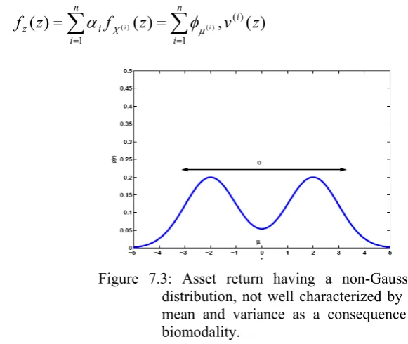
In seventh chapter, “Atzbergerţ’s extension of Markowitz portfolio selection”, represent one basic manner by which Markowitz’s theory for portfolio selection can be

extended to account for non-gaussian distributed returns. We then discuss how a model

incorporating information about the performance of the assets in different market regimes

over the holding period can be developed.

Most of the original results presented in this book were presented in very important

conferences and workshops. Also, we have to note the large list of references considered

elaborating this book.

I wish to acknowledge the teachers, colleagues, and reviewers who contributed to

earlier editions of this book and further to extend my appreciation for the guidance and

suggestions donated during its revision.

Gratitude is particularly due to Prof. DR. Vasile PREDA, Prof. DR. Ion V DUVA,

Acad. Marius IOSIFESCU, Dr. Ion M. STANCU-MINASIAN, DR. Miruna BELDIMAN,

DR. Roxana CIUMARA. I would also like to thank all the people who helped me. Above

Indonesia, H.E. Nuni Turnijati Djoko (Ambasador of the Republic of Indonesia in Bucharest

Romania), Islah Abdullah, Purno Wirawan, Sam E. Marentek, Hary Irawan, Pratiwi

Amperawati, Dedin M. Nurdin.

C

ONTENTS

Preface

Chapter 1 Introduction …………..……….. ……….... 1

Chapter 2 Some classes of stochastic problems ………... 7

2.1 Introduction ……… 7

2.2 Efficient solution concepts ……… 10

2.3 Relations between the efficient sets of several deterministic multiobjective programming problems ………... 13

2.4 Some relations between expected-value efficient solution, minimum-variance efficient solutions and expected-value standar-deviation efficient solutions ………... 19

2.5 Multicriteria problems ………. 20

2.6 Relations between classes of solutions for (P1), (P2) and (P3)….. 21

2.7 White’s approach multiobjective weighting factors auxiliary optimization problem for (P1), (P2) and (P3) ……….. 27

2.7.1 Introduction ………. 28

2.7.2 Transformations and auxiliary optimization problem associated to (P1), (P2) and (P3) ……….. 29

2.7.3 Non-convex auxiliary optimization problem 32 Chapter 3 Stochastic dominance …..………….……….. 40

3.1 Introduction ……… 40

3.2 Stochastic dominance ………. 42

3.4 Consistency with stochastic dominance ………. 45

Chapter 4 The dominance-constrained portfolio problem ………... 52

4.1 Introducere ……….. 52

4.2 Dominance-constrained . …….……… 53

4.3 Optimality and duality ……… 56

4.5 Spliting ….……….. 60

4.6 Decomposition …….………. 64

Chapter 5 A fuzzy approach to portfolio optimization ………. 68

5.1 Introduction ……….. 68

5.2 Fuzzy linear programming models ..………... 69

5.3 Interactive fuzzy programming ……….. 76

5.3.1 Interactive fuzzy linear programming algorithm ……… 78

5.4 Portfolio problem .………. 80

5.5 Case of fuzzy technological coefficient and fuzzy right-hand side numbers ……… 83

5.5.1 Case of fuzzy technological coefficients ……… 83

5.5.2 Portfolio problems with fuzzy technological coefficients and fuzzy right-hand-side numbers ………. 88

5.6 The modified subgradient method ……….. 93

5.7 Defuzzification and solution of defuzzificated problem ………. 96

5.7.1 A modified subgradient method to fuzzy linear programming ……… 96

5.7.2 Fuzzy decisive set method ..………... 98

5.8 Portfolio problem with fuzzy multiple objective ……….. 110

5.9.1 Problem formulation and the solution concept ………… 116

5.9.2 Solution algorithm ……….. 122

5.9.3 Basic stability nations for problem (FMOFP) ………. 125

5.9.4 Utilization of Kuhn-Tucker conditions corresponding to problem ………..………... 125

(

P

_λ

)

Chapter 6 A possibilistic approach for a portfolio selection problems .. 128

6.1 Introduction ……….. 128

6.2 Mean VaR portfolio selection multiobjective model with transaction costs ..………. 129

6.2.1 Case of downside-risk ..……….. 129

6.2.2 Case of proportional transaction costs model ………... 131

6.3 A possibilistic mean Var portfolio selection model …………... 131

6.3.1 Possibilistic theory. Some preliminaries ………. 132

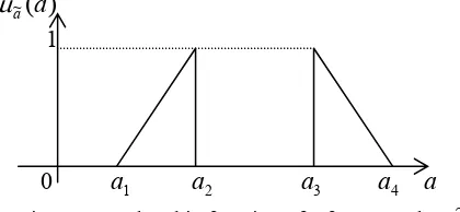
6.3.2 Triangular and trapezoidal fuzzy numbers …………... 133

6.3.3 Construction of efficient portfolios .……….. 135

6.4 A weighted possibilistic mean value approach ……….. 138

6.5 A weighted possibilistic mean variance and covariance of fuzzy numbers ………... 142

Chapter 7 An extention of Markowitz portfolio selection ……….. 146

7.1 Introduction ……….. 146

7.2 Gaussian mixture distribution ……… 148

7.3 An extention of the Markowitz portfolio theory ……….. 151

7.4 Portfolio selection problem (GM-PoS) ………... 152

Bibliography

….

……….……… 154

Acronyms & Abbreviations

………

174

Index

………..

175

C

HAPTER 1

INTRODUCTION

The problem of optimizing a portfolio of finitely many assets is a classical problem in

theoretical and computational finance. Since the seminal work of Markowitz [112] it is

generally agreed that portfolio performance should be measured in two distinct

dimensions: the mean describing the expected return, and the risk which measures the

uncertainty of the return. In the mean–risk approach, we select from the universe of all

possible portfolios those that are efficient: for a given value of the mean they minimize

the risk or, equivalently, for a given value of risk they maximize the mean. This

approach allows one to formulate the problem as a parametric optimization problem, and

it facilitates the trade-off analysis between mean and risk.

In the classical approach to portfolio selection, one often applies the theory of

expected utility that is derived from a set of axioms concerning investor behaviour as

regards the ordering relationship for deterministic and random events in the choice set.

The specific nature of the axioms that characterize the utility function is based on the

assumption that a probability measure can be defined on the random outcomes.

However, if we assume that the origins of these random events are not well known, then

the theory of probability proves inadequate because of a lack of experimental

information. In such instances, one has to approach the decision theory problem under

uncertainty using different mathematical tools. Further, the preference function that

describes the utility of the investor may itself be changing with the degree of uncertainty.

Moreover, one could postulate that the investor has multiple preference functions each of

which corresponds to a particular view on various factors that influence the future state

of the economy and the confidence with which it is held. Under these conditions, the

existing literature in the field of economic theory does not provide the investor with

sufficient tools to address the portfolio selection problem. The discussion above

highlighted potential difficulties one would encounter when addressing the portfolio

would be confronted with multiple utility functions. Each one of these utility functions

may be attributed to a particular market view being held and can be broadly described as

capturing the investor’s level of satisfaction if it turns out to be true. For instance, a fund

manager structuring a fixed-income portfolio may have only vague views regarding

future interest rate scenarios and these can broadly be described as being “bullish”,

“bearish” or “neutral”. Such views may arise out of the subjective and/or intuitive

opinion of the decision-maker on the basis of information available at the given point in

time. Under these circumstances, one might try to characterize the range of acceptable

solutions to the portfolio selection problem as a fuzzy set (see Bellman and Zadeh [9]).

In simple terms, a fuzzy set is a class of objects in which there is no clear distinction

between those objects that belong to the class and those that do not. Further, associated

with each object is a membership function that defines the degree of membership of the

object in the set. In this respect, fuzzy set theory provides a framework to deal with

problems in which the source of imprecision is the absence of sharply defined criteria of

class membership rather than the presence of random variables. This provides the point

of departure from probability theory, where the uncertainty arises from the random

nature of the environment rather than from any vagueness of human reasoning. In the

context of choosing optimal portfolios that target returns above the risk-free rate for

certain market scenarios while at the same time guaranteeing a minimum rate of return,

fuzzy decision theory provides an excellent framework for analysis. This is because the

nature of the problem requires one to examine various market scenarios, and each such

scenario will in turn give rise to an objective function. In the face of uncertainty, one will

not be able to assign a numerical value to the probability of these scenarios occurring.

Under this constraint, it is not clear how a suitable weighting vector can be determined to

solve the multi-objective optimization problem. One way to overcome this difficulty is to

use the membership function that arises in fuzzy decision theory to serve as a suitable

preference function for finding an ordering relation for the uncertain events. In fact, one

can describe the membership function as the fuzzy utility of the investor, which

describes the behaviour of indifference, preference or aversion towards uncertainty,

Mathieu-Nicot [115]. The advantage of using the membership function is that it does not

rely necessarily on the existence of a probability measure but rather on the existence of

The above arguments show how the portfolio selection problem under uncertainty can be

transformed into a problem of decision-making in a fuzzy environment Bellman and

Zadeh [9]. To do this, one has to model the aspirations of the investor on the basis of the

strength of the views held on various market scenarios through suitable membership

functions of a fuzzy set. For instance, a fund manager structuring a fixed-income

portfolio may have aspiration levels as to what the portfolio’s acceptable excess return

over the risk-free rate should be for those scenarios he/she considers more likely. The

concepts of fuzzy sets, fuzzy goals and fuzzy decision will be introduced and a fuzzy

multi-criteria optimization problem will be formulated.

As stated by Markowitz in [112,114), “The expected utility maxim appears reasonable

offhand. But so did the expected return maxim. Perhaps there is some equally strong

reason for decisively rejecting the expected utility maxim as well”.

The classical Markowitz model is

[ ]

( ) )

(x =Var R x

ρ

,

where

ρ

(

x

)

is the variance of the return, and

R

(

x

)

is total return. The mean–risk portfolio optimization problem is formulated as follows:

[

(

)

(

)

]

max

x

x

x∈X

μ

−

λρ

.

where R and X are defined in section 3.3.

Here,

λ

is a nonnegative parameter representing our desirable exchange rate of mean

for risk. If

λ

=0, the risk has no value and the problem reduces to the problem of maximizing the mean. If

λ

>0 we look for a compromise between the mean and the risk. The general question of constructing mean–risk models which are in harmony with

the stochastic dominance relations has been the subject of the analysis of the recent

papers Dentcheva and Ruszcynski [41,42], Rothschild and Stiglitz [155], Ogryczak and

Ruszczynski [127, 128].

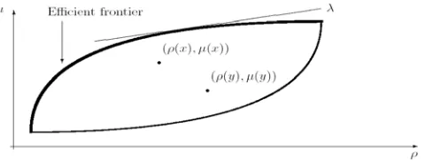
Portfolio selection is generally based on a trade-off between expected return and risk,

and requires a choice for the risk measure to be implemented. Usually, the risk is

evaluated by the conditional second-order moment, i.e., conditional variance or

volatility. This leads to the determination of the mean-variance efficient portfolio

(probability of failure), initially proposed by Roy [149] and then implemented by Levy

and Sarnat [100]. The efficient portfolio is one for which there does not exist another

portfolio that has higher mean and no higher variance, and/or has less variance and no

less mean at the terminal time T . In other words, an efficient portfolio is one that is Pareto optimal.

Notwithstanding its popularity, mean variance approach has also been subject to a lot of

criticism. Alternative approaches attempt to conform the fundamental assumptions to

reality by dismissing the normality hypothesis in order to account for the fat-tailedness

and the asymmetry of the asset returns. Consequently, other measures of risk, such as

Value at Risk (VaR), expected shortfall, mean absolute deviation, semi-variance and so on are used.

Another theoretical approach to the portfolio selection problem

- Stochastic dominance (Mosler and Scarsini, [121]), the concept of stochastic dominance

is related to models of risk-averse preferences Fishburn [52]. It originated from the

theory of majorization Hardly, Littlewood and Poya [70] for the discrete case, was later

extended to general distributions Quirk and Saposnik[146]; Hadar and Russel [66];

Hanoch and Levy [68]; Rothschild and Stielits [155], and is now widely used in

economics and finance (Levy [99]).

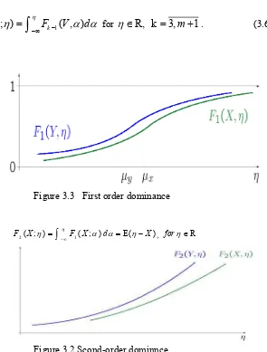
- The usual (first order) definition of stochastic dominance gives a partial order in the

space of real random variables. More important from the portfolio point of view is the

notion of second-order dominance, which is also defined as a partial order. It is

equivalent to this statement: a random variable R dominates the random variable Y if

)]

(

[

)]

(

[

u

R

E

u

Y

E

≥

for all non-decreasing concave functions u(·) for which these

expected values are finite. Thus, no risk-averse decision maker will prefer a portfolio

with return Y over a portfolio with return R.

- The stochastic optimization model with stochastic dominance constraints Dentcheva and

Ruszcynsk [42, 44], can be used for risk-averse portfolio optimization. We add to the

portfolio problem the condition that the portfolio return stochastically dominates a

reference return, for example, the return of an index. We identify concave

expected return modified by these utility functions, guarantees that the optimal portfolio

return will dominate the given reference return.

- Fuzzy set theory, since 1960s, has been widely used to solve many problems including

financial risk management. The concept of a fuzzy random variable is a reasonable

extension of the concept of a usual random variable in the many practical applications of

random experiments, where the implicit assumption of data precision seems to be an

inappropriate simplification rather than an adequate modeling of the real physical

conditions. By using fuzzy approaches, the experts’ knowledge and the investors’

subjective opinions can be better integrated into a portfolio selection model. Bellman and

Zadeh [9] proposed the fuzzy decision theory. Ramaswamy [14] presented a bond

portfolio selection model based on the fuzzy decision theory, Sudradjat and Preda [188]

presented on portfolio optimization using fuzzy decisions. The notion of a fuzzy random

variable (see for example, Kwakernaak [91], Puri and Ralescu [145], Kruse and Meyer

[89] provides a valuable model that is manageable in a probabilistic framework. Also,

the concept of fuzzy information presented by Zadeh [216] can formalize either the

experimental data or the events involving fuzziness. The concept of a fuzzy random

variable Puri and Ralescu [145] was defined as a tool for establishing relationships

between the outcomes of a random experiment and inexact data, Ostermark [128]

proposed a dynamic portfolio management model. Watada [201] presented another type

of portfolio selection model based on the fuzzy decision principle. The model is directly

related to the mean-variance model, where the goal rate for an expected return and the

corresponding risk described by logistic membership functions.

- In standard portfolio models uncertainty is equated with randomness, which actually

combines both objectively observable and testable random events with subjective

judgments of the decision maker into probability assessments. A purist on theory

would accept the use of probability theory to deal with observable random events, but

would frown upon the transformation of subjective judgments to probabilities. Tanaka

et al [194] give a special formulation of fuzzy decision problems by the probability

events. Carlsson et al [26] studied the portfolio selection model in which the rate of

return of security follows the possibility distribution. Sudradjat, Popescu and Ghica

[187] studied on possibilistic approach a portfolio selection problem. Applying

be easily introduced to the estimation of the return rates and (2) the reduced problem is

more tractable than that of the stochastic programming approach. Korner [86] pointed

out that the variability is given by two kinds of uncertainties: randomness (stochastic

variability) and imprecision (vagueness). Randomness models the stochastic variability

of all possible outcomes of an experiment. Fuzziness describes the vagueness of the

given or realized outcome. Kwakernaak [91] presented another explanation for the

difference between randomness and fuzziness. He pointed out that when we consider

an opinion poll in which a number of people are questioned, randomness occurs

because it is not known which response may be expected from any given individual.

Once the response is available, there still is uncertainty about the precise meaning of

the response.

The aim of this book is to examine methods for handling statistical problems

involving fuzziness in the elements of the random experiment, and serves as a point from

which to derive the Markowitz portfolio model in the presence of efficient solution

concepts for a stochastic multi-objective programming, develop portfolio optimization

model involving stochastic dominance constraints on the portfolio return and necessary

and sufficient conditions of optimality and duality, we develop portfolio optimization

using fuzzy decisions in concentrate on fuzzy linear programming, and finally we

consider a mathematical programming model with possibilistic constraint and we it solve

C

HAPTER 2

SOME CLASES OF STOCHASTIC PROBLEMS

2.1 Introduction

Stochastic programming deals with a class of optimization models and algorithms in

which some of the data may be subject to significant uncertainty. Such models are

appropriate when data evolve over time and decisions need to be made prior to observing

the entire data stream. For instance, investment decisions in portfolio planning problems

must be implemented before stock performance can be observed. Similarly, utilities must

plan power generation before the demand for electricity is realized. Such inherent

uncertainty is amplified by technological innovation and market forces. As an example,

consider the electric power industry. Deregulation of the electric power market, and the

possibility of personal electricity generators (e.g. gas turbines) are some of the causes of

uncertainty in the industry. Under these circumstances it pays to develop models in

which plans are evaluated against a variety of future scenarios that represent alternative

outcomes of data. Such models yield plans that are better able to hedge against losses

and catastrophic failures. Because of these properties, stochastic programming models

have been developed for a variety of applications, including electric power generation

(Murphy [124]), financial planning (Carino et al [23]), telecommunications network

planning (Sen et al [170]), and supply chain management (Fisher et al [51]), to mention a

few.

The widespread applicability of stochastic programming models has attracted

considerable attention from the OR/MS community, resulting in several recent books

(Kall and Wallace [77], Birge and Louveaux [16], Prekopa [138, 139]) and survey

articles (Birge [15], Sen and Higle [169]). Nevertheless, stochastic programming models

remain one of the more challenging optimization problems.

While stochastic programming grew out of the need to incorporate uncertainty in linear

and other optimization models (Dantzig [39], Beale [8], Charnes and Cooper [30]), it has

instance, decision analysis, dynamic programming and stochastic control, all address

similar problems, and each is effective in certain domains. Decision analysis is usually

restricted to problems in which discrete choices are evaluated in view of sequential

observations of discrete random variables. One of the main strengths of the decision

analytic approach is that it allows the decision maker to use very general preference

functions in comparing alternative courses of action. Thus, both single and

multi-objectives are incorporated in the decision analytic framework. Unfortunately, the need

to enumerate all choices (decisions) as well as outcomes (of random variables) limits this

approach to decision making problems in which only a few strategic alternatives are

considered.

These limitations are similar to methods based on dynamic programming, which also

require finite action (decision) and state spaces. Under Markovian assumptions the

dynamic programming approach can also be used to devise optimal (stationary) policies

for infinite horizon problems of stochastic control (see also Neuro-Dynamic

Programming by Bertsekas and Tsitsiklis [13]). However, DP-based control remains wedded to Markovian Decision Problems, whereas path dependence is significant in a

variety of emerging applications. Stochastic programming provides a general framework

to model path dependence of the stochastic process within an optimization model.

Furthermore, it permits uncountably many states and actions, together with constraints,

time-lags etc. One of the important distinctions that should be highlighted is that unlike

dynamic programming, stochastic programming separates the model formulation activity

from the solution algorithm. One advantage of this separation is that it is not necessary

for stochastic programming models to all the same mathematical assumptions. This leads

to a rich class of models for which a variety of algorithms can be developed. On the

downside of the ledger, stochastic programming formulations can lead to very large scale

problems, and methods based on approximation and decomposition become paramount.

A whole series of production processes, economic system of different types, and

technical objective is described by mathematical models which are multi-criteria

optimization problems (Steuer [177], Chankong and Haimes [29] and Stancu-Minasian

account simultaneously the influence of a number of contradictory external factors on

the system.

The most intensive development of the theory and the methods of detailed bibliographic

description of which is given in Zeleny [217] and Urli and Nadeau [196], are linear and

non linear multi-criteria optimization problems. Some classifications of the methods of

this type, oriented to the specific user, and multi-criteria optimization problems with

contradictory constraints were explored in are given (Salukavadze and Topchishvili

[166]). Very interesting results generalized into the general domination cone for different

classes of solutions of multi-criteria problem are given (Salukavadze and Topchishvili

[166]).

Now, one of the widely developing fields in multi-criteria optimization is its qualitative

theory; the most important results are given (Salukavadze and Topchishvili [166]).

Well-known algorithms can be modified and new theoritical results.

The objective of this chapter is to examine some properties of different classes of

multi-criteria optimization problem solutions.

Most real-life engineering optimization problems require simultaneous optimization of

more than one objective function. In these cases, it is unlikely that the same values of

design variables will results in the best optimal values for all the objectives. Hence, some

trade-off between the objectives is needed to ensure a satisfactory design.

As the system efficiency indices can be different (and mutually contradictory), it is

reasonable to use the multi-objective approach to optimize the overall efficiency. This

can be done mathematically correctly only when some optimality principle is used. We

use Pareto optimality principle, the essence of which is following. The multi-objective

optimization problem solution is considered to be Pareto-optimal if there are no other

solutions that are better in satisfying all of the objectives simultaneously. That is, there

can be other solutions that are better in satisfying one or several objectives, but they

2.2

Efficient solution concepts

Consider a model in which the design/decision associated with a system is specified via

vector x. Under uncertainty, the system operates in an environment in which there are uncontrollable parameters which are modeled using random variables. Consequently, the

performance of such a system can also be viewed as a random variable. Accordingly,

stochastic programming models provide a framework in which designs (x) can be chosen to optimize some measure of the performance (random variable). It is therefore natural to

consider measures such as the worst case performance, expectation and other moments

of performance, or even the probability of attaining a predetermined performance goal.

Let us consider the stochastic multi-objective programming problem Caballero, et al [21]

(

(

,

~

),...,

(

,

~

)

)

min

z

₁

x

c

z

_q

x

c

D

x∈ , (2.1)

where the following notations and assumptions

• there is a compact set D⊆Rn of feasible actions;

• n

x

∈

R

is thevector of decision variables of the problem and c~ is a random vector whose components are random continous variables, defined on the set

n

R

E

∈

. We assume given the family

F

of events (that is, subset of

E

) and the

distribution of probability P defined on

F

so that, for any subset of

E

,

A

⊂

E

,

F

∈

A

, the probability P(A) is known. Also, we assume that the distribution of probability P is independent of the decision variables

x

₁

,...,

x

_n;

• there are q objective functions

{

f

_k

(

⋅

)}

with

f

_k

(

x

)

∈

R

₊ for all x∈D and

c

~_{is a random vector whose components are random continuous variable;}

• it is required to find members of the efficient (vector minimal) set E of D with respect to the order relation

≤

on

R

q, where, by definition,

)}

(

)

(

)

(

)

(

,

:

{

x

D

y

D

f

y

f

x

f

y

f

x

E

=

∈

∈

≤

→

=

(2.2)

Let

z

_k

(

x

)

is the expected value of the kth objective function, and let

σ

_k

(

x

)

be its standard deviation,

k

∈

{

1

,...,

q

}

. Let us assume that, for every

k

∈

{

1

,...,

q

}

and for

relations between expected value standard deviation efficient solution and efficient

solutions.

Next the following definitions by Caballero, et al [21],

Definition 2.1 [21] Expected-Value Efficient Solution. The point x∈D is an expected-value efficient solution of the stochastic multi-objective problem if it is Pareto efficient to the following problem :

(

(

),...,

(

)

)

min

:

)

(

PE

z

₁

x

z

_q

x

D

x∈ .

Let E_PE be the set of expected-value efficient solution of the stochastic multi-objective problem.

Definition 2.2 [21] Minimum-Variance Efficient Solution. The point x∈D is a minimum-variance efficient solution for the stochastic multi-objective problem if it is a Pareto efficient solution for the problem :

(

( ),..., ( )

)

min

: )

(P 2 ₁2 x _q2 x

D

x

σ

σ

σ

_∈ .

Let _σ2

P

E

be the set of efficient solutions of the problem

(

P

σ

2

)

.

Definition 2.3 [21] Expected-Value Standard-Deviation Efficient Solution orE

σ

Efficient Solution. The point x∈Dis an expected-value standard-deviation efficient solution for the stochastic multi-objective programming problem if it is a Pareto efficient solution to the problem

(

(

),...,

(

),

(

),...,

(

)

)

min

:

)

(

PE

z

₁

x

z

_q

x

₁

x

_q

x

D

x

σ

σ

σ

_∈ .

Let

E

_PEσ be the set of expected-value standard-deviation efficient solutions of the stochastic multi-objective programming problem (2.1).

Now, we give the concepts of efficiency for two criteria of maximum probability. As we

will see next, in order to define these two concepts, the minimum-risk criterion (concept

of minimum-risk efficiency) and Kataoka criterion (efficiency in probability) are applied

respectively to each stochastic objective.

(

(

~

(

,

~

)

,...,

(

~

(

,

~

)

)

)

max

:

))

(

(

_{1 1 q q}

D

x

P

z

x

c

u

P

z

x

c

u

u

PRM

≤

≤

∈ ,

Let

E

_PRM(u) be the set of efficient solution for the problem (PMR(u)).

Definition 2.5 [21] Efficient Solution with Probabilities

β

₁

,...,

β

_q or

β

-Efficient

Solution. The point x∈D is an efficient solution with probabilities

β

₁

,...,

β

_q if there exist

u

∈

R

q such that

(

x

t

,

u

t

)

t is a Pareto efficient solution to problem:

))

(

(

PP

β

(

)

D

x

q

k

u

c

x

z

P

u

u

k k k

q u

x

∈

=

≥

≤

}

,

1

,

,

)

~

,

(

~

{

,...,

min

₁

,

β

Let

E

_PP(β)

⊂

R

n be the set of efficient solutions with probabilities

β

₁

,...,

β

_qfor the stochastic multi-objective programming problem (2.1).

It may be noted that these definitions of efficient solution are obtained by applying the

same transformation criterion to each one of the objectives separately (expected value,

minimum variance, etc.), and by building after word the resulting deterministic

multiobjective problem. In this sense, it is necessary to the following results.

Remark 2.1 The concepts of expected value, minimum variance, etc., weak and properly efficient solution can be defined in a natural way.

Remark 2.2The concepts of minimum-risk efficiency and

β

-efficiency require setting a priori a vector of aspiration levels u or a probability vector

β

. This implies that, in both cases, the efficient set obtained depends on the predetermined vectors in such a way that, in general, different level and proba bility vector give rise to different efficient sets,

). ( )

(

), ( )

(

' '

' '

β

β

β

β

PP PP

PRM PRM

E E

u E u E u

u

≠ ⇒

≠

≠ ⇒

≠

strictly increasing, the set of efficient solutions does not vary in problem if we substitute standard deviation for variance, White [209].

Remark 2.46 The efficiency in probability criterion is a generalization of the one presented by Goicoechea, Hansen, and Duckstein [63], who define the same concept taking the same probability

β

for all the stochastic objectives and with the probabilistic equality constraints taking the form

β

=

≤

}

)

~

,

(

~

{

z

_k

x

c

u

_k

P

.

This notion was introduced by Stancu-Minasian [179], considering the Kataoka problem

in the case of multiple criteria.

2.3

Relations between the efficient sets of several of deterministic

multiobjective programming problems

We present some relations between the efficient sets of several problems of deterministic

multi-objective programming problems. These results will be used later for analysis of

concepts of efficient solutions for multi-objective stochastic problems.

Considered

f

and

g

be vectorial functions defined on the same set

H

⊂

R

n with n

H

f

:

⊂

R

→

R

q and

g

:

H

⊂

R

n

→

R

q and let

α

,

γ

be nonnull vectors with q real components, that is,

α

,

γ

∈

R

q and

α

,

γ

≠

0

. Let us consider the following multiobjective problems:

(PD1)

min

(

f

1

(

x

),...,

f

q

(

x

),

1

(

g

1

(

x

)),...,

q

(

g

q

(

x

))

)

D

x∈

γ

γ

(2.3)

(PD2)

min

(

f

1

(

x

),...,

f

q

(

x

)

)

D

x∈ (2.4)

(PD3) min

(

1(g12(x)),..., q(gq2(x)))

)

D

x∈

γ

γ

(2.5)

with,

γ

∈

R

q,

γ

≠

0

. Let

E

₁

,

E

₂

,

E

₃ be the sets of weakly efficient, efficient, and

Theorem 2.1 We assume that

g

>

0

for every x∈D,. Then:

i1

E

2

∩

E

3

⊂

E

1

i2

E

2

∪

E

3

⊂

E

1w

i3

E

2w

∪

E

3w

⊂

E

1w

Proof:

(i₁)

x

∈

E

₂

∩

E

₃

Let us show that x∈E₁ by reductio ad absurdum. We assume that x∉E₁. Then, there

exist an

x

*

∈

D

such that

f

_k

(

x

*

)

≤

f

_k

(

x

)

and

γ

_k

(

g

_k

(

x

*

))

≤

γ

_k

(

g

_k

(

x

))

, for every

}

,...,

1

{

q

k

∈

, there being an

s

∈

{

1

,...,

q

}

for which the inequality is strict,

)

(

)

(

x

*

f

x

f

_s

<

_s or

γ

_s

(

g

_s

(

x

*

))

<

γ

_s

(

g

_s

(

x

))

.

Therefore, x∉E₂ or

x

∉

E

₃, since

γ

_k

(

g

_k

(

x

*

))

≤

γ

_k

(

g

_k

(

x

))

, implies

(

g

s0

(

x

*

))

≤

k k

γ

))

(

(

g

s0

x

k k

γ

, contrary to

x

∈

E

₂

∩

E

₃.

(i2 )

E

2

∪

E

3

⊂

E

1w

Let

x

∈

E

₂

∪

E

₃. Let us see that

x

∈

E

₁w by reductio de absurdum. We assume that

w

E

x

∉

₁ . Then, there exist a vector

x

*

∈

D

that weakly dominates x and so verifies

)

(

)

(

x

*

f

x

f

_k

<

_k and

γ

_k

(

g

_k

(

x

*

))

<

γ

_k

(

g

_k

(

x

))

, for every

k

=

{

1

,...,

q

}

. Thus, x∉E₂

and, since

(

g

(

x

*

))

(

g

(

x

))

k k k

k

γ

γ

<

, implies

(

g

s0

(

x

*

))

<

k k

γ

(

g

s0

(

x

))

k k

γ

,

x

∉

E

₃, contrary to

x

∈

E

₂

∪

E

₃.

(i3)

E

2w

∪

E

3w

⊂

E

1w

Let

x

∈

E

₂w

∪

E

₃w. Let us see that

x

∈

E

₁w by reductio de absurdum. We assume that

w

E

x

∉

₁ . Then, there exist a vector

x

*

∈

D

that weakly dominates the vector x and therefore verifies that

f

_k

(

x

*

)

<

f

_k

(

x

)

and

γ

_k

(

g

_k

(

x

*

))

<

γ

_k

(

g

_k

(

x

))

, for every

}

,...,

1

{

q

k

∈

. Thus,

x

∉

E

₂w and, since

(

g

(

x

*

))

(

g

(

x

))

k k k

k

γ

γ

<

, implies

<

))

(

(

g

s0

x

*

k k

γ

(

g

s0

(

x

))

k k

Thus, (i2) can be deduced from (i3) □

Now we consider the following problem

(

(

)

(

(

)),...,

(

)

(

(

))

)

min

f

₁

x

₁

g

₁

x

f

_q

x

_q

g

_q

x

D

x∈

+

α

+

α

(2.6)

where

α

=(

α

₁,...,

α

_q):R₊ →Rq.

Let E₄(

α

) and

E

₄G

(

α

)

denote the efficient solutions set and the properly efficient solutions set respectively for problem (2.6). We will now present some relations between

these sets and the set of efficient solutions and properly efficient solutions for problem

(PD1).

Theorem 2.2 [21]For

γ

=(

γ

₁,...,

γ

_q):R₊ →Rq,

α

=(

α

₁,...,

α

_q):R₊ →Rq, with

0

,

_k

≠

k

γ

α

and sign(

α

_k)=sign(

γ

_k),k =1,q, the following relation holds :

1

4( ) E

E

α

⊂ .

Proof: Let x∈E₄(

α

). We assume that x∉E₁. In this case, there is a solution

x

* that dominates the solution x, that is,

)

(

)

(

x

*

f

x

f

_k

≤

_k and

γ

_k

(

g

_k

(

x

*

))

≤

γ

_k

(

g

_k

(

x

))

, for every

k

∈

{

1

,...,

q

}

, and there

exist at least one

s

∈

{

1

,...,

q

}

for which the inequality is strict, that is,

)

(

)

(

x

*

f

x

f

_s

<

_s or

γ

_s

(

g

_s

(

x

*

))

<

γ

_s

(

g

_s

(

x

))

From this point onward, since

)

(

)

(

x

*

f

x

f

_k

≤

_k ,

γ

_k

(

g

_k

(

x

*

))

≤

γ

_k

(

g

_k

(

x

))

, implies

α

_k

(

g

_k

(

x

*

))

≤

α

_k

(

g

_k

(

x

))

,

the following inequalities are verified:

))

(

(

)

(

))

(

(

)

(

x

*

g

x

*

f

x

g

x

*

f

_k

+

α

_{k k}

≤

_k

+

λ

_{k k} , for every

k

∈

{

1

,...,

q

}

, (2.7)

))

(

(

)

(

))

(

(

)

(

x

g

x

*

f

x

g

x

f

_k

+

α

_{k k}

≤

_k

+

α

_{k k} , for every

k

∈

{

1

,...,

q

}

. (2.8)

From (2.7) and (2.8), we obtain

))

(

(

)

(

))

(

(

)

(

x

*

g

x

*

f

x

g

x

f

_k

+

α

_{k k}

≤

_k

+

α

_{k k} , for every

k

∈

{

1

,...,

q

}

.

In particular, for k =s, we have the results bellow:

(a) if

f

_s

(

x

*

)

<

f

_s

(

x

)

,

))

(

(

)

(

))

(

(

)

(

x

*

g

x

*

f

x

g

x

*

and the following inequality is obtained from (2.8):

))

(

(

)

(

))

(

(

)

(

x

*

g

x

*

f

x

g

x

f

_s

+

α

_{s s}

<

_s

+

α

_{s s} ;

(b) if

α

_s

(

g

_s

(

x

*

))

<

α

_s

(

g

_s

(

x

))

,

))

(

(

)

(

))

(

(

)

(

x

*

g

x

*

f

x

*

g

x

f

_s

+

α

_{s s}

<

_s

+

α

_{s s} ,

and since

f

_s

(

x

*

)

≤

f

_s

(

x

)

, we obtain

))

(

(

)

(

))

(

(

)

(

x

*

g

x

*

f

x

g

x

f

_s

+

α

_{s s}

<

_s

+

α

_{s s} .

Therefore, for every

k

∈

{

1

,...,

q

}

,

))

(

(

)

(

))

(

(

)

(

x

*

g

x

*

f

x

g

x

f

_k

+

α

_{k k}

≤

_k

+

α

_{k k} ,

and there is at least a subscript

s

∈

{

1

,...,

q

}

for which

))

(

(

)

(

))

(

(

)

(

x

*

g

x

*

f

x

g

x

f

_s

+

α

_{s s}

<

_s

+

α

_{s s} ,

which implies that the solution

x

* dominates the solution x; therefore, we reach a contradiction with the hypothesis of

x

* being the efficient solution to problem (2.6).

■

Next, we prove that, in some conditions, this relationship is hold for the set of properly

efficient solution. For this purpose, we define problems

P

_f,γg

(

λ

,

μ

)

and

P

_α

(

ξ

)

,

obtained by applying the weighting method to problems (2.3)-(2.6) respectively as

follows:

∑

₌

∈ +

q

k

k k k t

D x g

f f x g x

P

1

, ( , )): min ( ) ( )

( _γ

λ

μ

λ

μ

γ

,

)) ( )

( ( min :

)) ( (

1

x g x

f

P _{k k k}

q

k k D

x

ξ

α

ξ

α

∑

+

=

∈ .

We use the results available in the literature about the relationships between the

optimal solution to the weighting problem and the efficient solutions to the

multi-objective problem. Some results, see Chankong and Haimes [29], applied to problem

(a) If f and (

γ

₁g₁,...,

γ

_qg_q)t are convex functions, D is convex, and

x

* is a properly efficient solution for the multi-objective problem (2.3), there exist some weight

vector

λ

,

μ

with strictly positive components such that

x

* is the optimal solution

for weighted problem

P

_f,γg

(

λ

,

μ

)

.

(b) For each vector of weights with strictly positive components, the optimal solution to

the weighted problem

P

_f,γg

(

λ

,

μ

)

is properly efficient for the multi-objective

problem (P1).

Proposition 2.1 If

f

and

(

γ

₁

(

g

₁

),...,

γ

_q

(

g

_q

))

are convex functions, D is a convex set and there exist

α

=(

α

₁,...,

α

_q):R₊ →Rq ,

sign

(

α

_k

)

=

sign

(

γ

_k

)

, for every

}

,...,

1

{

q

k

∈

then

E

₄G

(

α

)

⊂

E

₁G.

Proof: If

f

and

(

γ

₁

(

g

₁

),...,

γ

_q

(

g

_q

))

are convex functions and if D is a convex set, then the set of properly efficient solutions to problems (PD1) and (2.6) are obtained from the

associated weighted problems for strictly positive weight vectors. We will prove that any

solutions to the optimization problem

P

_α

(

ξ

)

, with

ξ

>

0

, is a solution to problem

)

,

(

,γg

λ

μ

f

P

for some vector

(

λ

,

μ

)

>

0

.

Let

x

∈

E

₄G

(

α

)

. Then, given the established hypotheses, there exist a vector

ξ

>

0

for

which x is the solution for problem

P

_α

(

ξ

)

. Let us assume that, for every

0

,

},

,...,

1

{

≠

∈

q

k k

k

α

γ

. Then, we take

k

k

ξ

λ

=

,

μ

_k

=

ξ

_k

α

_k

/

γ

_k

,

λ

_k

,

μ

_k

>

0

,

Since

ξ

>

0

, we obtain that x is an optimal solution to problem

P

_f,λg

(

λ

,

μ

)

. For some

}

,...,

1

{

q

i

∈

if

α

_i

=

γ

_i

=

0

, then the proof would be the same, since in problem (2.3) the function

g

_i is not involved and since in problem (2.6) the function ith objective would be

f

_i. ■

Example 2.1. Let us consider the following problem:

,

0

,

,

1

9

.

/

),

,

(

max

2 2

,

≥

≤

+

y

x

y

x

t

s

y

x

y x

with

f

(

x

,

y

)

=

x

,

g

(

x

,

y

)

=

y

,

u

=

1

.

The set of efficient points for this problem is

{

(

x

,

y

)

t

∈

R

2

/

x

2

+

4

y

2

=

1

,

x

,

y

>

0

}

and is represented in Fig. 2.1.

We outline the solution of the problem

,

0

,

,

1

9

.

/

,

max

2 2

,

≥

≤

+

+

y

x

y

x

t

s

y

x

y

x

α

with

α

>0. For each fixed

α

>0, the optimal solution of the resulting problem is one of property efficient solutions to the original becriterion problem.

y

1

ε

D

3 x

Figura 2.1

Proposition 2.2 If

f

and

(

γ

₁

(

g

₁

),...,

γ

_q

(

g

_q

))

are convex functions, then

U

Ω ∈

⊂

α

α

)

(

4 1

G

G

E

E

,

with

Ω

=

{

α

=

(

α

₁

,...,

α

_q

)

:

R

₊

→

R

q

sign

(

α

_k

)

=

sign

(

γ

_k

),

k

=

1

,

q

}

.

Proof: As the previous case, the proof of the proposition is carried out by demonstrating that any solution to the problem

P

_f,γg

(

λ

,

μ

)

is a solution to the problem

P

_α

(

ξ

)

for

Consider

x

∈

E

₁G. Since f and (

γ

₁g₁,...,

γ

_qg_q)t areconvex functions, there exist vector

0

,

μ

>

λ

such that x is a solution to problem

P

_fug

(

λ

,

μ

)

. Because

ξ

,

μ

>

0

we put

k

k

λ

ξ

=

,

k k k

k

ξ

γ

μ

α

=

,

since

ξ

,

μ

>

0

, therefore we obtain that x is also a solution to the problem

P

_α

(

ξ

)

.

□

From Proposition 2.1 and Proposition 2.2, if

f

and (

γ

₁g₁,...,

γ

_qg_q)t are convex

functions and if

sign

(

α

_k

)

=

sign

(

γ

_k

)

,

α

_k

(

t

).

γ

_k

(

t

)

>

0

, for every

k

∈

{

1

,...,

q

}

, the sets of properly efficient solutions to problem (2.3) and (2.6) verify the following

properties:

a. Every properly efficient solution to problem (2.6) is properly efficient for problem

(2.3);

b. Setting

γ

∈

R

q, with nonnull components, the set of properly efficient solutions to problem (2.3) is a subset of the union in

α

of the set of properly efficient solutions

for problem (2.6).

2.4

Some relation between expected-value efficient solution,

minimum-variance efficient solution and expected-value standard deviation

efficient solution

Consider a problem (2.1) and sets efficient solution expected value (E_PE) minimum

variance (

E

_PEσ2), and expected value standard deviation (

E

_PEσ ) associated with the

problem. Let w _PEw

PE w

PE E E

E , _σ2, _σ be the sets of weakly efficient solutions associated with

the problems in Definitions 2.1-2.3, respectively.

If we consider

)

(

)

(

),

(

)

(

x

z

x

g

x

x

f

_k

=

_{k k}

=

σ

_k

2.5 Multi-criteria problems

Consider the following model of a multi-criteria optimization problem:

(

(

),...,

(

)

)

min

F

₁

x

F

_q

x

(2.8)

D

x∈ (2.9)

where D is a nonempty set of all feasible solution,

D

⊂

R

m;

F

₁

,...,

F

_q

:

D

→

R

. Stated briefly, a multi-criteria optimization problem consists in the choice of a particular

solution

x

*

∈

D

for which all of the utility functions F_k(x),k=1,q, simultaneously

approach bigger values or at least do not decrease.

Let us recall some concepts of multi-criteria optimization problem solutions; (Zeleny

[217] and Urli and Nadeau [196], Salukavadze and Topchishvili [166]).

Definition 2.6 The solution

x

P

∈

D

is called Pareto-optimal (or efficient) for the problem (2.8)-(2.9) if and only if, for every x∈D, the system of inequalities

)

(

)

(

_k P

k

x

F

x

F

<

,

k

=

1

,

q

,where at least one inequality is strict, is inconsistent.

Definition 2.7The solution

x

w

∈

D

, is called weakly efficient (or Slater-optimal) for the problem (2.8)-(2.9) if and only if, for every x∈D, the system of strict inequalities

)

(

)

(

_k w

k

x

F

x

F

<

,

k

=

1

,

q

, is inconsistent.

Definition 2.8 The solution

x

G

∈

D

, is called proper efficient (or Geoffrion-optimal) for the problem (2.8)-(2.9) if and only if it is a Pareto-optimal solution for the problem

(2.8)-(2.9) and there exists a positive number

θ

>0 such that, for each

k

=

1

,

p

, we have

θ

≤ −

− ( )]/[ ( ) ( )] )

(

[F x F x F xG F_j x

j G k

k ,

for some j such that F_j(x) > F_j(xG) where x∈D and

F

_k

(

x

)

<

F

_k

(

x

G

)

k

=

1

,

q

, is inconsistent.

Let Ew_j,

E

,

EG_j denoted the sets of weakly-efficient, efficient, and proper efficient

solutions, respectively, for the problem (2.8)-(2.9). It is obvious that

G j

Next we will studied some relations between the efficient sets of several problems of

deterministic multi-objective programming.

Let

f

and

g

be vectorial functions defined on the same set H ⊆Rn, with q

R

H

f

:

→

and

g

:

H

→

R

₊q. Let us consider the following multi-objective problems:

(P1)

min

(

f

₁

(

x

),...,

f

_q

(

x

),

u

₁

(

g

₁

(

x

)),...,

u

_q

(

g

_q

(

x

))

)

D

x∈ (2.10)

(P2)

min

(

f

1

(

x

),...,

f

q

(

x

)

)

D

x∈ (2.11)

(P3) min

(

u1(g10(x)),...,u (g 0(x)))

)

s q q s

D

x∈ (2.12)

with,

D

⊆

H

,

u

:

R

₊

→

R

q,

u

=

(

u

₁

,...,

u

_q

)

and

s

₀

>

0

a real number.

2.6 Relations between classes of solutions for (P1), (P2) and (P3)

We present some relations between the efficient sets of above considered deterministic

multi-objective programming problems. These results will be used later for analysis of

concepts of efficient solutions for multi-objective stochastic problems. These results

extend Section 2.4.

For

i

=

1

,

2

,

3

, let

E

_iw

,

E

_i

,

E

_iG