Weather and Infant Mortality in Africa
Masayuki Kudamatsu, Torsten Persson, and David Str¨omberg
∗August 16, 2016
Abstract
Using 50 retrospective fertility surveys from 28 countries and global me-teorological reanalysis data for 1957-2002, we estimate the causal impacts of malarious weather and growing-season rainfall on infant mortality across a considerably wide set of African locations. Relying on year-to-year devia-tions from the local monthly average pattern, we find that mortality rose by at least a quarter of the sample mean for infants born after droughts in arid climates, or after unusually long spells of malarious weather in low malaria-transmission areas. Our estimates imply that malarious weather explains at least 1.8% of infant mortality in Africa’s low malaria-transmission areas.
∗Kudamatsu: OSIPP at Osaka University, 1-31 Machikaneyama Toyonaka, Osaka, 560-0043
1
Introduction
To evaluate global policy responses to climate change, we must learn more about the impact of weather on important socioeconomic outcomes. Infant mortality in Africa is one such outcome. Despite a declining trend, the mortality rate of newborns in the sub-Saharan part of the continent still stands around 60 per 1,000 live births in 2013, ten times higher than prevailing rates in high-income countries (World Bank 2015).
Although mortality impacts of climate change have been widely discussed (Costello et al. 2009, Patz et al. 2005, Stern 2007), credible impact estimates to inform this discussion are very difficult to obtain for low-income, data-poor regions (Parry et al. 2007). This applies particularly to Africa, a region thought to be very vulnerable to climate change. Africa’s presumed vulnerability reflects that its adverse weather changes are likely to be substantial (IPCC 2014) and that its major production sec-tors are highly weather-dependent, as are its major diseases like malaria.
In this paper, we provide the estimates of how weather affects infant mortality in Africa by using micro data, and use these estimates to predict areas at risk for high infant mortality, 100 years down the line, under two different emission scenarios. Our empirical strategy has three distinctive features, which concernscale,structure, andsource of identification.
Scale We use a dataset with a massive number of observations at wide
geograph-ical coverage and high spatial resolution. For weather, we use data for all of Africa from meteorological reanalysis by a global atmospheric weather-forecasting model, on a 1.25×1.25degree earth grid (139 ×139 kilometers, at the equator) with a
six-hour frequency from 1957 to 2002. For infant mortality, we use micro data from 50 nationally representative retrospective fertility surveys, known as Demo-graphic and Health Surveys (DHS). These cover nearly one million live births, ob-served monthly, at more than 17,500 geo-referenced locations in 28 countries across Africa.
observe a large number of rare weather events, including droughts and unusually long spells of malarious weather in areas where malaria is not endemic.
Structure To use the data efficiently, we exploit prior structural knowledge on
how weather patterns link to infant mortality in Africa. The IPCC Report (Niang et al. 2014) and the Stern Review (Nkomo et al. 2011) list Africa’s main weather-related vulnerabilities: (i) droughts and floods, (ii) safe drinking water and sanita-tion, (iii) agriculture and food security, (iv) malaria, and (v) environmental conflicts and migration driven by food scarcity. These vulnerabilities are directly related to the most common death causes among children on the continent: malnutrition, malaria, and diarrhoea (Black et al. 2008, Black et al. 2010). While we know little about how weather affects drinking water, sanitation, or diarrhoea incidence, the previous research in public health and agricultural science inform us how specific weather conditions shape malaria transmission and crop yields.
In particular, we follow Tanser et al. (2003) in measuring malarious weather by four local temperature and rainfall conditions, which are necessary for the survival and growth of malaria vectors and parasites. We also measure the amount of rainfall in each location during the growing season, the weather condition most relevant for food security and scarcity. To isolate the impacts of malarious weather and growing-season rainfall from other weather impacts, we follow the recent climate-economy literature (see below) by controlling for the frequencies at which temperature and precipitation fall into different bins.
We believe that using structural indices of malarious weather and growing-season rainfall have two clear advantages over non-parametric or agnostic approaches. First, since our indices are guided by pre-existing research on weather-patterns linked to key mortality factors, they are likely to predict infant mortality in an effi-cient way. Second, since our indices capture structural mechanisms, they allow us to extrapolate the findings to out-of-sample areas or time periods.
Source of identification Studying the effects of climate change is plagued by
continental or global models of malaria-climate relationships ... fail to account for non-climatic determinants or the variation of specific climate-disease relationships among locations.” It is not feasible to control for all relevant drivers of infant mor-tality because average geographic and seasonal climate differences are correlated with numerous determinants of infant mortality. To tackle this problem, we follow the same approach as studies in the new climate-economy literature (see below), namely to identify the causal effects of weather shocks on infant mortality from ex-ogeneous deviations of local weather outcomes from their average monthly pattern.
Findings We uncover a set of new results. We find statistically and quantitatively significant effects of malarious weather in areas with low malaria transmission, where epidemiology studies have been very scarce (Desai et al. 2007). Compared to a typical year in these epidemic areas, malarious weather for more than six months in the year before birth makes infants 2.8 to 3.7 percentage points more likely to die in their first year of life. This additional death toll amounts to a quarter to a third of mean mortality in the sample. As for growing-season rainfall, infants in arid-climate regions of Africa face a risk of death 2.5 percentage points higher than in a typical year if they are born within a year after a drought. This effect is just over a quarter of the sample average. Even though these extreme weather events are very rare, these numbers are precisely estimated thanks to the large number of observations and the wide spatial coverage of the data.
By multiplying the sample frequencies of malarious weather spells with the es-timates of their impact (relative to the level of mortality in the absence of malarious weather), we obtain the average number of infant deaths due to these spells. Our estimates suggest that at least 1.8% of infant deaths can be attributed to malari-ous weather in Africa’s low malaria-transmission areas. A comparable estimate is absent in the epidemiology literature, as most malaria transmission surveys are conducted in high malaria-transmission areas (Desai et al. 2007).
Related work Our study is in line with the new climate-economy literature,
sur-veyed by Dell et al. (2014), in that we rely on random weather fluctuations around locality-specific average patterns. The impact of weather on mortality has recently been investigated by Deschˆenes and Greenstone (2011) and Barreca et al. (2016) for the United States, and by Burgess et al. (2013) for India. Deschˆenes et al. (2009) also look at the impact on birth weight.1 These studies non-parametrically estimate the impact of binned temperature realizations, and find that extremely high temper-atures raise general mortality, and reduce the birth weight of infants, respectively.2
The use of reanalysis data for weather – and growing-season rainfall as the condition relevant for crop yield – makes our paper related to Guiteras (2009), who studies how weather affects agriculture in India. The use of weather to predict disease environments echoes the approach taken by Alsan (2015).
Our study is also related to a large literature in public health and epidemiology, which investigates either how malaria and/or malnutrition responds to weather (e.g., Hay et al. 2009), or how infant health responds to malaria or malnutrition (e.g., Steketee et al. 2001, Black et al. 2008, Black et al. 2010). Unlike these studies, we estimate a direct causal link from weather conditions to infant mortality. Therefore, our impact estimates not only reflect pregnant women’s health conditions (the focus of these earlier studies). They also reflect health conditions among other members in the households of newborn babies, as well as behavioral changes by mothers and other household members in response to weather outcomes. This way, our estimated parameters may be of more immediate interest for the debate on the adverse impacts of climate change.
Roadmap In the following, Section 2 gives a general background on our data
sources and how we put the data together. Section 3 describes the details of our empirical approach, our measurement of malarious weather and growing-season rainfall, and our econometric specifications. Section 4 discusses our empirical
find-1See Deschˆenes (2012) for a review of the literature on the impact of temperature on health. 2Artadi (2006) estimates the impact of being born in rainy seasons and hungry seasons on infant
ings and robustness checks when it comes to the recent history of weather and infant mortality in Africa. Section 5 extrapolates these findings to the whole of Africa and to the future under two different scenarios for carbon-dioxide emissions. Section 6 concludes. The Appendix spells out some additional details on data construction, econometric strategy, and auxiliary evidence.
2
Data
This section describes our data and their sources.
Infant deaths To measure infant deaths, we pool together the retrospective fertility-survey component of 50 nationally representative Demographic and Health Surveys (DHS) (Corsi et al. 2012) in 28 African countries. Appendix Table A.1 lists the sur-veys used in the analysis. Women aged 15 to 49 in sampled households are asked about the month and year of each live birth they gave in the past, whether the child died after birth and, if so, the age at death in months. From this information, we define a binary indicator whether the child died at an age of 12 months or less.3
These 50 surveys cover nearly 1.2 million live births to about 300,000 mothers in 1957-2002, the period for our weather data. Since we exploit year-to-year varia-tion by calendar month and locavaria-tion, we drop observavaria-tions with imputed birth dates, leaving us with 962,471 live births by 269,754 mothers in 17,568 geo-referenced survey clusters (villages or town districts).4
Note that our measure of infant mortality does not include stillbirths. Appendix Section A.1 provides further detail on the DHS surveys. The section also discusses possible biases due to data accuracy and finds that these are likely to be small. Section 4.5 discusses possible sample-selection bias due to endogenous fertility and maternal mortality.
3We include reported deaths at 12 months because of a peak at that age in the distribution of ages
at death. Excluding deaths at 12 months does not qualitatively change our estimation results.
4One could argue that mortality of babies with missing birth date may be lower because mothers
Weather To gauge local temperature and precipitation, we use the ERA-40 data
archive (Uppala et al. 2005), obtained from meteorological re-analysis.5 The
re-analysis was carried out by a global atmospheric weather-forecasting model on a
1.25×1.25degree earth grid (about 139 x 139 km at the equator) with a six-hour
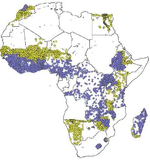
frequency for the period from 1 September 1957 to 31 August 2002. We aggregate the original six-hourly data to monthly data on temperature and total precipitation. Then, we match each DHS survey cluster to its corresponding ERA-40 grid cell by ArcGIS’s Spatial Join tool, resulting in 743 grid cells covering 17,568 DHS clusters. Figure 1 illustrates the geographical coverage of these data and shows that a wide range of African regions are included in our sample.
We expect ERA-40 to contain among the best weather data for Africa, especially for its arid and semi-arid areas. The climate model makes observations from data-sparse regions more realistic and reliable, as weather follows physical laws almost linearly at a six-hour time scale. This advantage is larger from the time when global satellite data (fed into the climate model to predict the atmospheric state) becomes available: in 1973 and, at higher frequency, in 1979. About 88% of the births in our sample occur after 1978.
Most importantly, the precipitation data in ERA-40 do not depend on rainfall gauge data, which is particularly coarse and low-quality in Africa, but instead on the climate model and the estimated state of the atmosphere.6 A comparison of
rainfall data from ERA-40 and gauge data (where available) by Zhang et al. (2013) suggests that the ERA-40 data have less bias in the arid and semi-arid areas of Africa, where the departures from regular seasonal fluctuations – our main source of identification – are the largest.
5See Appendix Section A.2 for how re-analysis in ERA-40 is conducted. Also see Auffhammer
et al. (2013) for an account of re-analysis directed to economists.
6Due to the well-known difficulty of predicting the precise location of convective rainfall (i.e.
thunderstorms), the forecast may fail to predict the exact amount of rainfall in a precise location in a particular six-hour period. Aggregation in time (to a month) and space (to1.25×1.25degrees),
3
Structural Measurement and Estimation
This section first explains how we exploit prior knowledge on weather patterns that are likely to impact infant mortality in Africa to produce indices measuring malarious weather condition and growing-season rainfall. Then, it discusses our econometric specification.
3.1
Malarious Weather Conditions
The monthly malaria index Our goal is to construct a binary indicator for weather
conditions in a particular month being suitable for malaria transmission. We do so by adapting a parsimonious weather-based index of malarious conditions for Africa proposed by Tanser et al. (2003), which is in turn based on the work by the Mapping Malaria Risk in Africa (MARA) project (Craig et al. 1999).7 These authors validate
their index against 3,791 laboratory-confirmed parasite-ratio surveys of one-month duration across Africa conducted between 1929 and 1994. They find that, if the index indicates malarious weather, then 99% of the surveys indeed report malaria prevalence. If the index indicates the absence of malarious weather, 67% of the surveys report malaria prevalence.
Specifically, we define our binary monthly index as follows. Letτ be the (run-ning) month of birth andg the ERA-40 grid cell. Our index for locationg in birth monthτ, denoted byZg,τ, takes a value of one if the following four conditions are satisfied:
(a) Average monthly rainfall during the past 3 months (the birth month and the two proceeding months) is at least 60mm;
(b) Rainfall in at least one of these months is at least 80 mm;
(c) None of the past 12 months (the birth month or the previous 11 months) has an average temperature below5◦C; and
7Appendix Section A.3 discusses the original index of Tanser et al. (2003) in detail and how our
(d) The average temperature in the past 3 months exceeds the sum of19.5◦C and
the standard deviation of monthly average temperature in the past 12 months.
Ifanyof these conditions fails, our malaria index turns to zero. Conditions (a) and (b) ensure the availability of breeding sites for the vector and sufficient soil moisture for vectors to survive; (c) rules out the death of vectors, as this happens quickly at lower temperatures; and (d) allows parasites to become infectious inside the vector’s body before the vector dies.8 The required threshold of temperature in
condition (d) goes up with the standard deviation of monthly temperature because, after a cold winter, the populations of parasites and vectors need to be quickly regenerated to a level sufficient for malaria transmission. Using the ERA-40 data, we then calculate the malaria index for each grid cell and month.9
The year prior to birth Infants are known to have a reduced sensitivity to malaria
during the first few months of life (Maegraith 1984). On the other hand, malaria in pregnancy10is known to raise the likelihood of low birth-weight, a major risk factor
for infant death (McCormick 1985).11
For these reasons, we focus on malarious weather in the year prior to birth as a determinant of infant death. For an infant born in cellg in month t, we define the key independent variable in our estimation of the impact of malarious weather:
zg,t =
t X
τ=t−11
Zg,τ , (1)
8The vector obtains a parasite by biting a malaria-infected person. But it takes time for the
parasite to become infectious and thus for the vector to transmit malaria by biting another person. Higher temperature both shortens the time required for the parasite to become infectious and helps the vector survive long enough.
9Dropping separately each of the four conditions, we find conditions (a) and (d) to be the most
relevant ones to predict infant death.
10See Desai et al. (2007) for a recent and extensive review of the medical literature on malaria in
pregnancy.
11On top of a higher likelihood of low birth-weight, babies born to mothers with a malaria-infected
where Zg,τ is the monthly malaria index in ERA-40 cellg at (running) month τ, defined above. In words, zg,t measures how many months in the year before birth weather conditions are conducive to malaria transmission.
Although we expect maternal malaria infection to be the major channel through which malarious weather affects infant death, our 12-month index of malarious weather,zg,t, may also capture the effect of malaria infection by other members of the mother’s household or their behavioral change in response to malarious weather. Consequently, our estimates should be interpreted as the full impact of malarious weather, not as the impact of maternal malaria infection.
Appendix Section A.4 discusses whether malarious weather after birth matters for infant mortality. We find no significant effects on infant mortality of in-life shocks.
Malaria zones We strongly expect the impact of variations in malarious weather
conditions on infant mortality to be larger in areas where malaria transmission is low. Where malaria is endemic, adults develop partial immunity from repeated in-fections since childhood and thus avoid symptoms such as fever and anemia. Where malaria is seasonal or epidemic-prone, however, most adults lack such partial im-munity. In these areas, people of all ages remain susceptible to the full range of clinical effects. Hence we expect weather shocks to matter more in these malaria-epidemic areas.12
We use our monthly index of malarious weather to identify epidemic and en-demic areas. If the average annual number of malarious months in each ERA-40 grid-cell during 1957-2002 is more than zero and up to four, we call the grid-cell
epidemic. If it is larger than four, we call itendemic.13 Finally, if it is zero, we call
itnon-malarious. Figure 1 shows the distribution of these three malaria zones by color. This map corresponds well to the distribution of parasite infection in malaria
12Due to the lack of partial immunity, pregnant women get sicker once infected with malaria in
epidemic areas than in endemic areas. One of the symptoms of malaria, fever, is known to increase the chance of premature delivery and of infant death (Luxemburger et al. 2001). Since malaria mortality in general is known to be much higher in epidemic areas (Kiszewski and Teklehaimanot 2004), the death of a pregnant mother’s household members may be more likely, possibly affecting her baby’s survival through income loss or the mother’s psychological stress.
maps based on cross-sectional clinical observations (Hay et al. 2009).
3.2
Growing-Season Rainfall
Measuring growing seasons Alongside malaria, crop yields are the major
chan-nel through which weather outcomes shape human life in Africa. Most African countries are agricultural economies – in 2004, some 55% of people on the conti-nent were employed in agriculture (Frenken 2005, Table 2), and many more depend on agriculture in other indirect ways. As transportation infrastructure in Africa is poorly developed, most people are largely dependent on the local yields of subsis-tence crops, or on cash crops for income to buy food.14
Crop yields in Africa’s non-tropical areas are crucially dependent on the sea-sonal rains in thegrowing season. Irrigation plays a minor role, especially in Sub-Saharan Africa – only 6.4% of cultivated land was irrigated in 2004 (Frenken 2005, Table 12).
We therefore use total precipitation during the location-specific growing season to capture the weather impact on infant mortality via crop yields. We first determine annual growing seasons in each ERA-40 grid cell. To do so, we use a satellite measure of plant growth derived by the TIMESAT program (J¨onsson and Eklundh 2004) to process the bi-weekly NDVI index (Tucker et al. 2005) at a resolution of
8×8kilometers from 1982 onwards (see Appendix Section A.5 for more detail).
We then average the start and end dates of the annual growing seasons in each location, to avoid the endogeneity of each year’s growing season to socioeconomic determinants of infant mortality. Finally, using the precipitation data in ERA-40, we calculate the total annual amounts of rainfall during the location-specific average growing season.15
To validate total rainfall during the growing season as a measure of food avail-ability, we compare it to monthly crop prices in the following 12 months for se-lected African locations. We find that low growing-season rainfall indeed predicts
14Herbst (2000, Table 5.3) reports that the road density for the median African country around
the year of 1997 is merely 0.07 kilometers per square kilometers of land.
15In areas where there are two growing seasons per year, we use every odd growing season in our
high crop prices in the following year quite well (see Appendix Section A.6 for detail).
The year prior to birth Food availability prior to birth is more important than
availability after birth for infant survival. On the one hand, maternal malnutrition poses a major risk for infant health (Black et al. 2008). A lack of food during pregnancy diminishes the intake of calories and important micro-nutrients, which negatively affects the growth of the fetus in utero. This raises the risk of low birth-weight, which in turn raises the risk of infant death through birth asphyxia and infections (McCormick 1985). On the other hand, most African infants are breast-fed, and thus have lower mortality risk than those who obtain non-breast milk liquid or solid food during the first six months of life (see, e.g., Black et al. 2008, Table 4).16
We therefore focus on food availability during the 12-month period prior to birth, in an analogous fashion to our analysis on malarious weather. Since rainfall during the growing season does not affect crop yields until the end (harvest) of the season, we match growing-season rainfall to each birth month in the following way. First, we divide total rainfall in the growing season equally into the following 12 months. Then, we sum the monthly allocations of growing-season rainfall over the 12 months before each birth, to approximate available crop yields for the mother and her household in this period.
The above procedure effectively produces the weighted sum of total rainfall during the two previouscompletedgrowing seasons. Putting it mathematically, let
rg,t1 and rg,t2 be total rainfall during the last and second-to-last completed growing seasons before running montht in grid cellg. For infants born in that month and grid cell, we assign the following growing-season rainfall index:
rg,t ≡ωg,trg,t1 + (1−ωg,t)r
g,t
2 , (2)
16One might think that food availability after the birth of a child is important for his or her mother
with the weight given byωg,t = (t−hg,t)/12, wherehg,t is the running month of
the last harvest.
Growing-season rainfall is likely to have a nonlinear impact on infant mortality. Susser (1991), for example, reviews studies on the relationship between maternal nutrition and birth weight and concludes that nutritional intake by mothers signif-icantly affects birth weight only in famine conditions. To capture this non-linear impact, we create a drought index fromrg,tin the following way. For each ERA-40 grid cell, we calculate the mean and standard deviation ofrg,t. Based on these mo-ments, we create the drought index as a dummy variable, whenrg,tis more than two standard deviationsbelowits mean. This index is similar to the Standardized Pre-cipitation Index (McKee et al. 1993), a widely-used measure of drought, but based onrg,trather than monthly rainfall.17
It is important to note that this growing-season rainfall index captures not only maternal nutritional intake but also other channels through which crop yields influ-ence the survival of newborns. For example, crop yields affect the mother’s house-hold income, which may affect prenatal health-care access. Low crop yields may cause conflicts (e.g., Miguel et al. 2004), which may in turn affect the survival of infants. Our purpose in this paper is to estimate the total impact of growing-season rainfall on infant mortality.
Climate zones We allow one unit of growing-season rainfall to translate into dif-ferent amounts of crop yields by splitting the sample according to climate, to which people adapt by crop choice (e.g., drought-resistant millet and sorghum in arid ar-eas). We rely on the K¨oppen classification, which distinguishes climate types by monthly mean temperature and precipitation, as well as the latitude (Peel et al. 2007). Using these criteria and our ERA-40 data, we subdivide all DHS clusters into two climate zones: rainy(rainforest, monsoon, savannah and temperate cli-mates), andarid(steppe and desert climates) areas. This classification is shown in Figure 2. Arid-climate zones largely overlap with epidemic-malaria zones in Figure 1.
17We also consider an analogous flood index (i.e. two standard deviations above the mean).
3.3
Summary Statistics
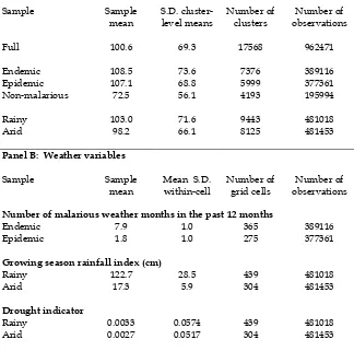
Table 1 reports summary statistics for infant mortality and the two weather vari-ables, by malaria zones and climate zones.
Panel A shows that average infant mortality in the sample is 108.5 and 107.1 per 1,000 live births in malaria endemic and epidemic areas, respectively. These numbers are much higher than in non-malarious areas (72.5 per 1,000). The higher death toll in malarious areas may reflect differences in socioeconomic determinants of infant survival from non-malarious areas. Our estimation results help us disen-tangle the mortality by malarious weather from that due to other causes (see Section 4.4).
Panel B of Table 1 reports summary statistics on the number of malarious months in the year before birth, by malaria zone. Mothers in endemic areas are on average exposed to 7.9 months of malarious weather conditions, with the stan-dard deviation of 1.0 months. In epidemic areas, the corresponding numbers are 1.8 and 1.0 months. Mean-adjusted variability is thus much higher in epidemic areas.
Panel B also shows the mean and standard deviation of the growing-season rain-fall index: 122.7 and 28.5 for the rainy climate zone, and 17.3 and 5.9 for the arid climate zone. Mean-adjusted variability is clearly larger for the arid climate zone.
3.4
Econometric Specification
Identifying variations To identify the causal effects of weather outcomes, we
will only use temporary deviations in weather outcomes from their average monthly pattern in each location. On top of the regular seasonal cycle, temperature and rain-fall in Africa fluctuate considerably from year to year, especially in arid and semi-arid areas. The fluctuations partly reflect chaotic weather dynamics over horizons beyond a couple of weeks. They also reflect hard-to-predict, medium-term fluc-tuations in air pressure associated with the Southern Oscillation.18 The warming
phase (El Nino) is generally associated with wetter-than-normal weather in East Africa during March-May, but less rainfall than normal in parts of South and
Cen-18The time series pattern of these fluctuations during the past century are analyzed and discussed
tral Africa during December-February, with opposite patterns during the cooling phase (La Nina).
Estimation equation We estimate the impact of malarious weather and
growing-season rainfall on infant death by versions of the following equation for infantiborn in cluster c(located in grid cellg and country x) in calendar months of calendar yeary:
In this expression, the dependent variableyi,c,s,yis the infant-death indicator. This is multiplied by 1,000 to allow the estimated coefficients to be interpreted as changes in the number of death per 1,000 live births (the conventional unit for infant-mortality statistics). As we control for cluster-by-month fixed effects,µc,s, the source of iden-tification is the deviation from the average seasonal pattern in each location, i.e., the random component of weather outcomes. Year-fixed effects are allowed to differ by country (ηx,y), to control for non-parametric trends in national health systems, poli-cies, or economic conditions, which could conceivably be related to local weather outcomes.19 In addition, we control for grid-cell specific linear trends, δgGs,y, to
allow for sub-national trends.
Independent variables The key independent variables areMg,s,yandRg,s,y.Mg,s,y
is the vector of malarious weather variables (constructed from our 12-month index,
zg,s,y, defined in equation (1)).Rg,s,yis a vector of growing-season rainfall variables
(defined in Section 3.2) that capture the weather impact on crop yields, including the (log) growing season rainfall index (ln(rg,t+ 1)),20the drought index, and their
19For example, Kudamatsu (2012) finds democratization has reduced infant mortality in
sub-Saharan Africa while Bruckner and Ciccone (2011) find negative rainfall shocks led to democrati-zation in Africa.
20The growing season rainfall index is transformed in the logarithm term after adding one. The
interactions with the rainy climate-zone indicator.
To isolate the impacts of malarious weather conditions and growing-season rain-fall from other weather impacts, we control for two additional sets of weather vari-ables. First,Tg,s,yis a vector of the number of days in the past 12 months in which
daily average temperature falls in various categories (below 16◦C, 16-18◦C, 18
-20◦C, ...,34-36◦C, and above36◦C).21 These variables capture the impact of daily
temperatures in the year up to birth in a flexible fashion, following the approach in Deschenes and Greenstone (2011), Barreca et al. (2016), and Burgess et al. (2013) among others.
Second, Pg,s,yis a vector of dummies for the past 12-month total precipitation
falling in various categories (less than 500mm, 500-550mm, 550-600mm, ..., 950-1000mm, and above 1000mm).22 These variables capture the potentially nonlinear
impact of total rainfall in the year up to birth.23
For inference, the error term,εi,c,s,y, is clustered at the ERA-40 grid-cell level to compute the standard errors, because weather variables are measured at the grid-cell level and likely to be serially correlated. To allow for spatial correlations across time (i.e., the correlation of weather at one location in the current month and at another location in the subsequent months), we also adopt an alternative scheme where we cluster standard errors at the country by malaria zone (endemic, epidemic, and non-malarious).
To summarize, our parameters of interest α and β measure how many more infants per 1,000 live births die by one unit change in the related weather variables. Since we control for cluster-month fixed effects, we are identifying these parameters from the deviation within each cluster from its site-specific monthly mean.
tail.
21The most frequent category26-28◦C is omitted to avoid multicollinearlity.
22The category in which the sample average 12-month total precipitation falls is omitted to avoid
multi-collinearity.
23Following Burgess et al. (2013), we also specify the impact of the past 12 month total
4
Past Weather and Infant Mortality
This section presents our results regarding the effects on infant mortality of malari-ous weather conditions and growing-season rainfall.
4.1
Full-Sample Results
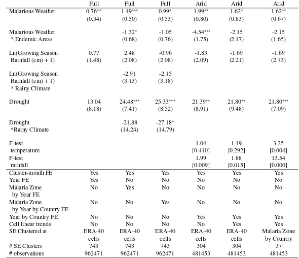
Columns (1) to (3) of Table 2 report the full sample results. For the impact of malarious weather, we estimate its linear impact by using our 12-month index in this table. Column (1) controls for year fixed effects and cluster-month fixed ef-fects. One additional month of malarious weather within the year before birth is estimated to increase infant mortality by 0.76 per 1,000 live births. The coefficients on growing season rainfall variables are both imprecisely estimated.
In column (2), we allow year fixed effects to differ across the three malaria zones (endemic, epidemic, and non-malarious) and interact the 12-month malaria weather index with the indicator for malaria-endemic areas, to see if partial im-munity developed in these areas mitigates the impact of malarious weather shocks. The coefficient on the interaction term is negative and significant at the 10% level. It suggests that one additional month of malarious weather has a nearly zero effect on infant death in endemic areas while 1.49 more infants per 1,000 live births die in epidemic areas due to one extra month of malarious weather (significant at the 1% level).
In column (2), we also interact the growing season rainfall variables with the indicator for rainy climate zones (tropical and temperate climates), to allow for differential impacts by crop choice in response to the climate. The drought in arid areas is estimated to increase infant mortality by 24.5 per 1,000 live births, and this estimate is statistically significant at the 1% level. In rainy areas, this effect appears to be muted, although the estimate is noisy.
shocks because, for example, infections spread between neighboring areas. For growing-season rainfall variables, the estimated impact of droughts in arid areas is comparable to column (2), now amounting to 25.3 extra infant deaths per 1,000 live births. The size of the impact is equivalent of more than a quarter of the sample mean infant mortality in arid climate zones. On the other hand, such a large impact is absent in rainy areas.
These full-sample results show that infants in epidemic areas are more likely to die if they are born after the longer spell of malarious weather than usual while those in endemic areas are not. Given this finding, we focus on the epidemic areas in more detailed analysis in Section 4.3 below. However, it is important to note that our result does not imply that in malaria-endemic areas malarious weather is not a large risk factor for infant death. Our identification of the impact hinges on the deviation from the average seasonal pattern of malaria transmission. As year-to-year variation in seasonal malaria transmission for endemic areas is not very large (as discussed in Section 3.3), most malaria-induced infant deaths are likely absorbed by the cluster-month fixed effects.
Another takeaway message from the full-sample results is that growing-season rainfall affects infant survival in arid climate zones when its amount is severely smaller than the normal year. In the next subsection, we check the robustness of this finding and discuss its implications.
4.2
Impacts of Growing-Season Rainfall
In columns (4) to (6) of Table 2, we restrict the sample to arid climate zones and check the robustness of our finding that the severe lack of growing-season rainfall raises infant mortality by as much as a quarter of the sample mean.
Column (4) controls for Tg,s,y (temperature bin variables) and Pg,s,y (rainfall
season rainfall thus affect infant mortality over and above the statistically significant impact of the past 12-month rainfall.
Column (5) further controls for the ERA-40 cell-specific linear trends. The estimated coefficient on the drought index changes little. Column (6) uses the same specification as in column (5) except that standard errors are clustered at the country-by-malaria-zone level, to allow spatial correlations in the error term across ERA-40 cells. The standard error for the drought coefficient is smaller than in col-umn (5).
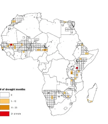
By definition, the drought is a rare event. Therefore, our finding could be driven by a few outliers. However, the incidence of these droughts is not concentrated in a particular period or in a specific area. Out of 69,303 months in which we observe at least one birth in the arid areas, droughts occurred in 181 months. Figure 3 shows the spatial distribution of the number of such drought months across arid areas. As the figure shows, the droughts from which we identify our estimates are quite evenly spread over the various African regions in the arid climate zone. Consequently, the estimated impact of droughts on infant mortality is not driven by an outlier.24
In summary, these arid-sample results show that infants in arid areas are more likely to die, by as much as 22% of the sample mean mortality, if they are born after a severe lack of growing-season rainfall in the previous two completed growing seasons. In Appendix Section A.6, we show that the severe lack of growing-season rainfall raises staple crop prices by 9.5% in the arid areas. This finding suggests that the shortage of nutritional intake due to drought is one mechanism through which droughts raise infant mortality. Taken together, our finding is consistent with the argument by Susser (1991), as discussed in Section 3.2, that it is only in famine conditions that nutritional intake by mothers significantly affects birth weight (and consequently the survival of newborns).
24In comparison, it is noteworthy that the vast majority (99%) of deaths (of all ages) due to
4.3
Impacts of Malarious-Weather Fluctuations
Our analysis for malarious weather in epidemic areas starts by relaxing the linear impact assumption. From the 12-month index of malarious weather, we construct five dummy variables for the number of months with malarious weather in the year before birth being zero, one or two, three or four, five or six, and more than six. We use these dummies as the key independent variables,Mg,s,y in equation (3).
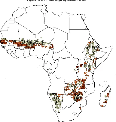
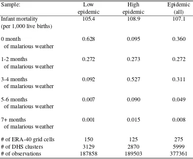
We also split the epidemic area into two subgroups,low-epidemicareas (where average malarious weather months are more than zero and up to two) and high-epidemicareas (average malarious weather months more than two and up to four).25
The spatial distribution of these two subgroups is illustrated in Figure 4. Table 3 shows the summary statistics by these two subsamples.
Low-epidemic areas Columns (1) to (3) of Table 4 restrict the sample to
low-epidemic areas. The distribution of exposure to malarious weather conditions in this subsample is highly skewed to the left. While over 60% of the births have no malaria exposure at all during the preceding year, about 1% of births are exposed to five or more months of malaria (see Table 3).
In the empirical specification for low-epidemic areas, we omit the dummy for 1 to 2 malarious months in the year before birth. Consequently, the coefficients on the dummies for the number of malarious weather months should be interpreted as how many more infants die per 1,000 live births relative to a typical year (with 1 or 2 malarious months).
In Table 4, column (1) controls for the growing-season rainfall variables and their interactions with the rainy climate-zone indicator (Rg,s,y in equation (3)) as
well as cluster-month and country-year fixed effects. To isolate the impact of malar-ious weather conditions from other weather impacts, column (2) additionally con-trols for Tg,s,y (the temperature bins), and Pg,s,y (the precipitation bins). Column
(3) further controls for linear trends specific to each ERA-40 cell, which is our preferred specification represented by equation (3).
25We have also tried to distinguish areas with seasonal and unstable malaria, based on the standard
Results are similar across these three columns. A malaria “epidemic” with more than 6 months of malarious weather in the year before birth kills 36.1 additional infants per 1,000 in their first year of life, statistically significant at the 5% level, according to the estimates in column (3). Since average infant mortality in this subsample is 107 per 1,000, this is an increase by about a third. An epidemic with 5-6 malaria months raises infant deaths by 12.5 per 1000, though this impact is not precisely estimated.
For low-epidemic areas, the temperature-bin variables are not jointly significant, while the precipitation-bin variables are jointly significant at the 1% level.
High-epidemic areas In columns (4) to (6) of Table 4, we restrict the sample to high-epidemic areas, where nearly 10 percent of births have no exposure to malar-ious weather in the preceding year, while 1% are exposed to 7 or more malaria months (Table 3). For this subsample, we omit the dummy for 3 to 4 malarious months in the year before birth, so the coefficients on the dummies should be in-terpreted as how many more infants die per 1,000 live births relative to the typical year (with 3 or 4 malarious months). Otherwise, the specification for columns (4), (5) and (6) is the same as for columns (1), (2), and (3), respectively.
Similarly to the low-epidemic sample, we find that zero or very little exposure is associated with much lower infant-mortality rates than above 6 months exposure. However, the estimated impact size now depends on the specification. Comparing column (4) to columns (5) and (6), the size of coefficients on the malarious-weather index dummies increases in absolute terms by controlling for temperature- and rainfall-bin variables, each of which is jointly significant at the 5% level. Adding the weather-bin variables one set at a time (results not reported), we find that the precipitation-bin variables drive the change in the size of estimated coefficients. Very little (large) amount of rainfall increases (decreases) infant mortality, which reduces the absolute size of the coefficients on the malarious-weather index dum-mies in column (4). Since we control for growing-season rainfall variables, the precipitation-bin variables might pick up the impact on infant mortality via the availability of safe drinking water.
con-vincingly isolate the impact of malarious weather conditions from other weather impacts. This is hence our preferred specification. Compared to the average year, a more than 6 month spell of malarious weather raises infant deaths by an additional 26.7 per 1,000 live births, nearly a quarter of the sample mean mortality of 108.9 per 1,000. A year without any malarious weather and with 1-2 malarious months reduces infant deaths by similar magnitude: 7.0 and 8.3 per 1,000, respectively.
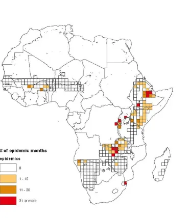
Frequency and location of malaria epidemics We will refer to the
longer-than-usual spell of malarious weather with a sizeable impact on infant death asmalaria epidemics (i.e., 5 or more malaria months in the low-epidemic area; 7 or more months in the high-epidemic area). Out of 63,317 months in which we observe at least one birth in epidemic areas, malaria epidemics hit 844 months, suggesting that the results are not driven by very few observations. Figure 5 shows the number of months with malaria epidemics on a map, analogous to Figure 3 for droughts. These events occurred in a variety of locations, but with a certain concentration to East Africa, especially the mountainous regions around the Great Rift Valley.
4.4
Average Effects of Malarious Weather
Given that columns (3) and (6) of Table 4 show a similar level of mortality across epidemic areas when the number of malarious weather months is at most two, in column (7) we pool low and high epidemic areas and estimate the impact of three-to-four, five-to-six, and more than six months of malarious weather, relative to an at most two-month long spell. The set of controls is the same as in columns (3) and (6). The estimated impacts are 5.12 per 1,000 live births for three-to-four months of malarious weather, 2.89 for five-to-six months, and 25.41 for more than six months. These coefficients are jointly significant at 1% level (with an F-statistic of 3.86).
areas (107.1 per 1000 live births).
The epidemiology literature, surveyed by Steketee et al. (2001), attributes 3-8% of infant mortality in malaria-endemicregions to maternal infection of malaria. Our results supply related estimates for the regions where malaria transmission is only seasonal.
In addition to these new substantive findings, we also make a methodological contribution. The methodology in Steketee et al. (2001) differs from ours in sev-eral aspects. Their study relies on two randomized control trials in rural Gambia (Greenwood et al. 1992) and Malawi (Steketee et al. 1996), which evaluate the impact of chemoprophylaxis treatment to pregnant women. These two areas may not be representative of all malaria-endemic regions of Africa. In addition, insuffi-cient statistical power due to a limited number of observations forces the underlying studies to focus on birth weight rather than infant mortality. The causal impact on birth weight is then multiplied with the correlation coefficient between birth weight and infant mortality, plausibly introducing omitted-variable bias. Our study, on the other hand, is immune to these issues because of the large number of observations, the wide spatial coverage of the data, and the reliance on deviations of weather outcomes from the annual seasonal pattern to identify the direct impact on infant mortality.
Our estimates, however, donotconcern the long-run effect of becoming malar-ious or non-malarmalar-ious due to climate change. In the long run, behavior may change in response to the absence or emergence of malaria, which may change average health and income levels, for example.
4.5
Additional Results and Robustness
Heterogeneous impacts Following the medical literature summarized in Appendix
Sample selection bias Annual weather fluctuations relative to the normal
sea-sonal pattern are plausibly exogenous to socioeconomic conditions. But the esti-mated coefficients on the indices of malarious weather and growing-season rainfall may still be biased, if the type of women who give live birth changes with weather realizations.26 Appendix Section A.8 deals with this sample-selection issue by esti-mating equation (3) with the dependent variable replaced by three characteristics of mothers or births known to be associated with higher infant mortality in develop-ing countries (Hobcraft et al. 1985). Specifically, we consider whether the mother: (i) gave her previous birth within 24 months, (ii) was under 20 years old, (iii) was uneducated. The results suggest that, in one case, the maximal bias is no greater than 6.4% of the estimated extra infant deaths by a long spell of malaria infection risk. In the other cases, sample-selection bias cannot account for changes in infant mortality by more than 0.47 per 1,000 live births.
Harvesting Some of the estimated impacts of weather shocks on infant mortality may be due to ‘harvesting’: some frail babies may just die a little earlier than they would in the absence of weather shocks. Research on the mortality impacts of high temperature in the US does indeed find evidence for harvesting (e.g., Deschˆenes and Moretti 2009).
To check how much of our estimated impacts of weather shocks can be at-tributed to harvesting, we restrict the sample to those babies who survive the first year of their life. Then, we investigate how much lower under-five mortality is for those children whose mother experienced weather shocks during the year before birth. More specifically, we use the specifications in column (6) of Table 2 (for the drought impact) and in columns (3) and (6) of Table 4 (for the malarious weather impact), with the dependent variable replaced by the indicator of death at 60 months old or younger in a sample restricted to those who do not die at 12 months old or younger.
Appendix Tables A.6 and A.7 report the results. The drought in terms of growing-season rainfall before birth reduces under-five mortality in arid areas by 12.7 per
26Our data exhibit sample selection bias if annual weather fluctuations affect the likelihood of
1,000 babies who survive the first year, although this point estimate is not signifi-cantly different from zero. Since the average infant mortality in arid areas is 98.2 per 1,000 live births, the drought before birth reduces under-five mortality by 11.5 per 1,000 live births, 53% of the estimated impact of drought on infant mortality.
For the impact of malarious weather, under-five mortality in low-epidemic areas and high-epidemic areas is lower by 7.8 and 3.0, respectively, per 1,000 babies who survive the first year of life if there are seven or more months of malarious weather in the year before birth, although neither of the point estimates is significantly dif-ferent from zero. Given the average infant mortality in these two areas (105.4 and 108.9 per 1000 live births), under-five mortality is reduced by 7.0 and 2.6, respec-tively, per 1,000 live births due to the epidemic before birth, amounting to 19.3% and 9.9% of the estimated impacts on infant mortality.
In high-epidemic areas, 2 or less months of malarious weather before birth re-duce under-five mortality by less than 2 per 1,000 babies surviving the first year
(not significantly different from zero), suggesting that the survival during the first year of life due to the absence of malarious weather before birth does not simply postpone the death during childhood.
Overall, harvesting can not fully explain the impact of weather shocks on infant mortality that we have estimated. While nearly half of the drought impact may be explained by harvesting, at the very most a fifth of the malarious weather impacts can be explained by harvesting.27
5
Future Climate and Infant Mortality
Our estimates in Section 4 strongly suggest that extreme weather events – large shortages of growing-season rainfall in arid areas and long spells of malarious weather in epidemic areas – had sizeable impacts on infant mortality in Africa’s
27We also look at the impacts on death at 24, 36, and 48 months old or younger, among those
recent history. However, these two extreme weather events may have only affected sparsely populated areas. They may also become less frequent in the future un-der climate change. In this section, we investigate the magnitude of impacts of the extreme weather events in spatial and temporal dimensions.
5.1
Methodology
We predict the total number of infant deaths due to the weather events, and its spatial distribution acrossallof Africa during two twenty-year periods: 1981-2000 and 2081-2100. For each period, the prediction involves three steps: (1) assume that our impact estimates also apply out of sample both space-wise and time-wise; (2) predict the total number of births in each weather-grid cell; and (3) compute the number of weather events from the output of climate models. Appendix Section A.9 gives more details on our methodology.
Step (1) involves the use of the impact estimates reported in column (5) of Table 2 for drought in arid areas and in column (7) of Table 4 for malarious weather, respectively. The underlying assumption is that there will be no adaptation in the way people deal with drought and malarious weather. While we acknowledge its unsatisfactory nature, our estimates will guide us about the importance of adaptation by showing the severity of impacts in the case of no adaptation.
In Step (2), we predict the monthly number of births in each 1.125 x 1.125 de-gree cell (the unit of observation for the future weather data) during 1981-2000 and 2081-2100, by using the spatial population data for 1990, 1995, and 2000 (CIESIN/CIAT 2005), together with country-level annual population growth and crude birth rates for 1981-1990 (World Bank 2015) and with predictions for 2000-2100 (United Nations Population Divisions 2011). Although these estimates are bold extrapolation, they help us figure out whether extreme weather event strike more populated areas or not.
Phase 5 (CMIP5): a high-emissions scenario (RCP8.5) and a mid-range emissions scenario (RCP4.5) (Taylor et al. 2012). These forecasts are derived from the EC-EARTH climate model, which is close to the one used in the ERA-40 re-analysis. To resolve the difference in the spatial resolution of weather data between ERA-40 and CMIP5, we match CMIP5 cell centroids with ERA-40 grid cells.
5.2
Estimated Effects and Areas at Risk
Malarious weather We focus on areas that never fall into the malaria-endemic
zone, because our historical estimates (Table 4, column 7) do not apply to endemic regions. To identify these areas, we use the CMIP5 data for monthly temperature and rainfall to obtain a spatial distribution of the monthly malaria index during the second half of this century (2051-2100). Based on the average annual number of malarious months during these 50 years, we classify all African locations into non-malarious, epidemic, and endemic zones. We then focus on areas that never fall into the endemic zone: the colored areas in Figure 6. For these cells, we estimate changes in the number of infant deaths attributed to malarious weather from the pe-riod of 1981-2000 to 2081-2100. These areas comprise 30.4% of the total estimated births in 2100 and are exposed to 12.5% and 12% of the birth-weighted absolute changes in the number of malarious months under the midrange and high emissions scenarios, respectively.
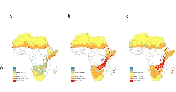
Figure 6 reports these predicted changes under the mid-range-emissions sce-nario (part a) and under the high-emissions scesce-nario (part b). To ease the compar-ison, part c shows how many more infants will die due to malarious weather if we go from mid-range to high emissions.
never-endemic areas is estimated to be 140,050 during 1981-2000. This number will moderately increase to 165,794 under the mid-range emissions scenario while it will shoot up to 711,617 under the high-emissions scenario. Even though the mid-range emissions scenario has warmer weather than now, it also has a different spatial distribution of rainfall, shifting malaria-enabling rains towards areas with a smaller population. A significant portion of the excess infant mortality is due to extreme spells of more than six months of malarious weather. Of the 711,617 predicted deaths in the high-emissions scenario, 117,344 are due to these spells.
Note that these estimates do not reflect the total death toll from malarious weather across Africa. Some non-endemic areas in the 20th century will become endemic while part of the 20th-century endemic areas will be non-endemic. Such areas are excluded from these estimates. Still, our analysis indicates the magnitude of changes in the number of deaths by malarious weather in large parts of Africa.
Droughts Predicting the death by droughts in the future requires the following
assumption on adaptation to climate change: the area that becomes an arid climate zone will adapt to the new climate via crop choice. Thus, the drought threshold for growing-season rainfall is based on the weather pattern during 2050-2100. We report only the spatial distribution of drought deaths during 1981-2000 and under the two climate change scenarios during 2081-2100. Unlike in our analysis on malarious weather, we do not look at changes in the number of deaths by drought in each location because the arid climate zone changes by period and by emission scenario.
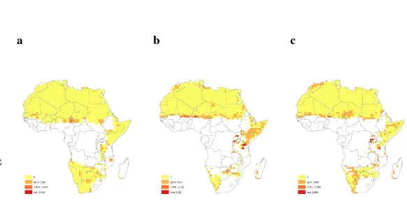
Figure 7 shows the spatial distribution of droughts for 1981-2000 (part a) and the two 2081-2100 climate scenarios (parts b and c). The colored areas indicate the arid climate zone in each period and climate scenario. The yellow areas have no drought during the respective 20-year period. The yellow-orange, red-orange, and red areas have the death by drought up to 1,000, between 1,000 and 2,000, and over 2,000, respectively.
populated areas. It is also visible in the Sahel region. The mid-range-emission sce-nario leaves densely populated southern Somalia and eastern Kenya at risk, while the high-emission scenario instead predicts droughts along the sparsely populated Namibia-Botswana border.
The estimated number of infant deaths due to droughts is only 10,848 during 1981-2000. It will jump to 49,883 under mid-range emissions 2081-2100, but only to 34,533 under high emissions. Our analysis illustrates how a higher level of emis-sions may not necessarily translate into a larger total number of infant deaths, be-cause of the geographical interaction between weather patterns and population den-sities.
6
Conclusions
We combine survey data for nearly one million live births at more than 17,500 geo-referenced locations in 28 African countries with meteorological reanalysis data in high spatial resolution from 1957 to 2002. The size of the data set helps us estimate precisely how outcomes as rare as infant death are affected by rare weather events, such as droughts in arid areas and long spells of malarious weather in areas with seasonal malaria transmission.
Substantially, we study weather effects on infant mortality in areas with low
malaria-transmission, where epidemiology studies have been very scarce, and find that these effects are likely to be non-negligible. The effect of malarious weather in malaria-epidemic regions amounts to 1.8% of sample-mean infant mortality. This can be compared to estimates of 3-8% of infant mortality in the malaria-endemic regions obtained by Steketee et al. (2001).
Our calculations suggest that the areas most exposed to climate risk depend crucially on the extent of future emissions. Along the stretch of land from western Tanzania to Zambia, for example, a high-emission scenario points to increased in-fant deaths due to malarious weather, while such deaths will fall from today’s level in a mid-range scenario.
illustrates a general and under-appreciated point: the effects of climate change on human health are likely to reflect not only average future weather patterns but also future weather variability.
Methodologically, we demonstrate how to use the estimated causal impact of temporary weather shocks to gauge the aggregate continent-wide impacts of spe-cific weather conditions, such as those leading to malaria epidemics.
We also showcase how to use estimated health impacts together with future climate scenarios to predict how climate change may expose certain areas to high risks of large health hazards, due to the interaction of future weather extremes and the spatial distribution of population.
References
[1] Alsan, Marcella. 2015. “The Effect of the TseTse Fly on African Develop-ment.”American Economic Review, 105(1): 382-410.
[2] Artadi, Elsa V. 2006. “Going into Labor: Earnings vs. Infant Survival in Rural Africa.” Unpublished paper.
[3] Auffhammer, Maximilian, Solomon M. Hsiang, and Wolfram Schlenker. 2013. “Global Climate Models and Climate Data: A User Guide for Economists.”Review of Environmental Economics and Policy, forthcoming.
[4] Barreca, Alan, Karen Clay, Olivier Deschˆenes, Michael Greenstone, and Joseph S. Shapiro. 2016. “Adapting to Climate Change: The Remarkable De-cline in the U.S. Temperature-Mortality Relationship over the Twentieth Cen-tury.”Journal of Political Economy, 124(1): 105-59.
[5] Black, Robert E., Lindsay H. Allen, Zulfiqar A. Bhutta, Laura E. Caulfield, Mercedes de Onis, Majid Ezzati, Colin Mathers, and Juan Rivera. 2008. “Ma-ternal and Child Undernutrition: Global and Regional Exposures and Health Consequences.”Lancet, 371(9608): 243-260.
Richard Cibulskis, Thomas Eisele, Li Liu, and Colin Mathers. 2010. “Global, Regional, and National Causes of Child Mortality in 2008: A Systematic Analysis.”Lancet, 375(9730): 1969-1987.
[7] Brown, K. H., and Kathryn G. Dewey. 1992. “Relationships Between Ma-ternal Nutritional Status and Milk Energy Output of Women in Developing Countries.” InMechanisms Regulating Lactation and Infant Nutrient Utiliza-tion, eds. M. F. Picciano and B. L¨onnerdal. New York: Wiley-Liss, pp. 77-95.
[8] Bruckner, Markus, and Antonio Ciccone. 2011. “Rain and the Democratic Window of Opportunity.”Econometrica, 79(3): 932-947.
[9] Burgess, Robin, Olivier Deschenes, Dave Donaldson, and Michael Green-stone. 2013. “The Unequal Effects of Weather and Climate Change: Evidence from Mortality in India.” Unpublished paper.
[10] Centre for Research on the Epidemiology of Disasters. 2013. EM-DAT: The International Disaster Database. www.em-dat.be.
[11] CIESIN/CIAT. 2005. Gridded Population of the World, Version 3 (GPWv3). Palisades, NY: Socioeconomic Data and Applications Center (SEDAC), Columbia University. Available at http://sedac.ciesin.columbia.edu/gpw.
[12] Corsi, Daniel J., Melissa Neuman, Jocelyn E. Finlay, and S. V. Subramanian. 2012. “Demographic and Health Surveys: A Profile.”International Journal of Epidemiology41 (6): 1602-1613.
[13] Costello, Anthony, Mustafa Abbas, Adriana Allen, Sarah Ball, Sarah Bell, Richard Bellamy, Sharon Friel, et al. 2009. “Managing the Health Effects of Climate Change: Lancet and University College London Institute for Global Health Commission.”Lancet373 (9676): 1693-1733.
[14] Craig, Marlies H., Robert W. Snow, and David le Sueur. 1999. “A Climate-Based Distribution Model of Malaria Transmission in Sub-Saharan Africa.”
[15] Dell, Melissa, Benjamin F. Jones, and Benjamin A. Olken. 2014. “What Do We Learn from the Weather? The New Climate-Economy Literature.”Journal of Economic Literature, 52(3): 740-98.
[16] Desai, Meghna, Feiko O ter Kuile, Franc¸ois Nosten, Rose McGready, Kwame Asamoa, Bernard Brabin, and Robert D. Newman. 2007. “Epidemiology and Burden of Malaria in Pregnancy.”Lancet Infectious Diseases, 7(2): 93-104.
[17] Deschˆenes, Olivier. 2012. “Temperature, Human Health, and Adaptation: A Review of the Empirical Literature.” NBER Working Paper w18345.
[18] Deschˆenes, Olivier, and Michael Greenstone. 2011. “Climate Change, Mor-tality, and Adaptation: Evidence from Annual Fluctuations in Weather in the US.”American Economic Journal: Applied Economics3 (4): 152-185.
[19] Deschˆenes, Olivier, Michael Greenstone, and Jonathan Guryan. 2009. “Cli-mate Change and Birth Weight.”American Economic Review Papers & Pro-ceedings, 99(2): 211-17.
[20] Deschˆenes, Olivier, and Enrico Moretti. 2009. “Extreme Weather Events, Mortality, and Migration.”Review of Economics and Statistics, 91(4): 659-81.
[21] Frenken, Karen, ed. 2005.Irrigation in Africa in Figures: AQUASTAT Survey, 2005. Rome: FAO.
[22] Greenwood, A.M., J.R.M. Armstrong, P. Byass, R.W. Snow, and B.M. Green-wood. 1992. “Malaria Chemoprophylaxis, Birth Weight and Child Survival.”
Transactions of the Royal Society of Tropical Medicine and Hygiene 86 (5): 483-485.
[23] Guiteras, Raymond. 2009. “The Impact of Climate Change on Indian Agricul-ture.” Unpublished paper.
[25] Herbst, Jeffrey. 2000. States and Power in Africa: Comparative Lessons in Authority and Control. Princeton, N.J.: Princeton University Press.
[26] Hobcraft, J. N., J. W. McDonald, and S. O. Rutstein. 1985. “Demographic Determinants of Infant and Early Child Mortality: A Comparative Analysis.”
Population Studies39 (3): 363-385.
[27] IPCC. 2014.Climate Change 2014: Impacts, Adaptation, and Vulnerability.
[28] J¨onsson, Per and Lars Eklundh. 2004. “TIMESAT – A Program for Analyzing Time-series of Satellite Sensor Data.”Computers and Geosciences, 30: 833-845.
[29] Kiszewski Anthony and A. Teklehaimanot A. 2004. “A Review of the Clin-ical and Epidemiologic Burdens of Epidemic Malaria.”American Journal of Tropical Medicine and Hygiene, 70:128-135
[30] Kudamatsu, Masayuki. 2012. “Has Democratization Reduced Infant Mortality in Sub-Saharan Africa? Evidence from Micro Data.”Journal of the European Economic Association, 10(6): 1294-1317.
[31] Le Hesran, Jean Yves et al. 1997. “Maternal Placental Infection with Plas-modium Falciparum and Malaria Morbidity during the First 2 Years of Life.”
American Journal of Epidemiology, 146(10): 826-831.
[32] Luxemburger, Christine, Rose McGready, Am Kham, Linda Morison, Thein Cho, Tan Chongsuphajaisiddhi, Nicholas J. White, and Francois Nosten. 2001. “Effects of Malaria during Pregnancy on Infant Mortality in an Area of Low Malaria Transmission.”American Journal of Epidemiology, 154(5): 459-465.
[33] Maegraith, Brian. 1984. Adams and Maegraith: Clinical Tropical Diseases. 8th ed. Oxford: Blackwell Scientific.
[35] McKee Thomas B., Nolan J. Doesken, and John Kleist. 1993. “The Relation-ship of Drought Frequency and Duration to Time Scales.” InEighth Confer-ence on Applied Climatology, Anaheim, CA, 179-184.
[36] Miguel, Edward, Shanker Satyanath, and Ernest Sergenti. 2004. “Economic Shocks and Civil Conflict: An Instrumental Variables Approach.”Journal of Political Economy,112(4): 725-753.
[37] Murray, Christopher J. L., and Alan D. Lopez, eds. 1996.The Global Burden of Disease: A Comprehensive Assessment of Mortality and Disability from
Diseases, Injuries, and Risk Factors in 1990 and Projected to 2020. Cam-bridge, MA: Harvard University Press.
[38] Niang, I., O.C. Ruppel, M.A. Abdrabo, A. Essel, C. Lennard, J. Padgham, and P. Urquhart. 2014. “Africa.” In: Climate Change 2014: Impacts, Adaptation, and Vulnerability. Part B: Regional Aspects. Contribution of Working Group
II to the Fifth Assessment Report of the Intergovernmental Panel on Climate
Change, Barros, V.R., C.B. Field, D.J. Dokken, M.D. Mastrandrea, K.J. Mach, T.E. Bilir, M. Chatterjee, K.L. Ebi, Y.O. Estrada, R.C. Genova, B. Girma, E.S. Kissel, A.N. Levy, S. MacCracken, P.R. Mastrandrea, and L.L. White (eds.) (Cambridge University Press), pp. 1199-1265.
[39] Nkomo, J. C., A. O. Nyong, and K. Kulindwa. 2011. “The impacts of climate change in Africa: final draft.” The Stern Review on the Economics of Climate Change.
[40] Owens, Stephen, G. Harper, J. Amuasi, G. Offei-Larbi, J. Ordi, and B.J. Bra-bin. 2006. “Placental Malaria and Immunity to Infant Measles.”Archives of Disease in Childhood, 91(6): 507 -508.
[42] Patz, Jonathan A., Diarmid Campbell-Lendrum, Tracey Holloway, and Jonathan A. Foley. 2005. “Impact of Regional Climate Change on Human Health.”Nature438 (7066): 310-317.
[43] Peel, Murray C., Brian L. Finlayson, and Thomas A. McMahon. 2007. “Up-dated World Map of the K¨oppen-Geiger Climate Classification.” Hydrology and Earth System Sciences, 11(5): 1633-1644.
[44] Snow, Robert W., Eline L. Korenromp, and Eleanor Gouws. 2004. “Pediatric Mortality in Africa: Plasmodium Falciparum Malaria as a Cause or Risk?”
American Journal of Tropical Medicine and Hygiene, 71(2 suppl): 16-24.
[45] Steketee, Richard W., Jack J. Wirima, and Carlos C. Campbell. 1996. “De-veloping Effective Strategies for Malaria Prevention Programs for Pregnant African Women.”American Journal of Tropical Medicine and Hygiene55 (1 Suppl): 95-100.
[46] Steketee, RW, BL Nahlen, ME Parise, and C Menendez. 2001. “The Burden of Malaria in Pregnancy in Malaria-Endemic Areas.” American Journal of Tropical Medicine and Hygiene64 (1 Suppl): 28-35.
[47] Stern, Nicholas. 2007.The Economics of Climate Change: The Stern Review. Cambridge University Press.
[48] Susser, Mervyn. 1991. “Maternal Weight Gain, Infant Birth Weight, and Diet: Causal Sequences.” American Journal of Clinical Nutrition, 53(6): 1384-1396.
[49] Taylor, Karl E. Ronald J. Stouffer, and Gerald A. Meehl. 2012. “An Overview of CMIP5 and the Experiment Design.”Bulletin of the American Meteorolog-ical Society, 93: 85-498.
[50] Tanser, Frank C, Brian Sharp, and David le Sueur. 2003. “Potential Effect of Climate Change on Malaria Transmission in Africa.”Lancet,362: 1792-1798.
2005. “An Extended AVHRR 8-km NDVI Dataset Compatible with MODIS and SPOT Vegetation NDVI data.” International Journal of Remote Sensing
26(20): 4485.
[52] United Nations Population Division. 2011.World Population Prospects: The 2010 Revision. Available at esa.un.org/unpd/wpp/unpp/panel indicators.htm
(accessed on 21 October 2012).
[53] Uppala, Sakari M. et al. 2005. “The ERA-40 Re-analysis.”Quarterly Journal of the Royal Meteorological Society,131(612): 2961-3012.
[54] World Bank. 2015. World Development Indicators. Available at data-bank.worldbank.org/data/home.aspx (Accessed on 9 November, 2015).
[55] Zhang, Quiong, Heiner K¨ornich, and Karin Holmgren. 2013. “How Well Do Reanalyses Represent the Southern African Percipitation.”Climate Dynamics, 40(3): 951-962.
Figure 1: The spatial distribution of observations and malaria zones.
Figure 2: Climate zones
Figure 3: Number of Drought Months in the Sample
Figure 4: Low and High Epidemic Areas
Figure 5: Number of Malaria Epidemic Months in the Sample
a
b
c
Figure 6: Predicted Changes in Number of Infant Deaths by Malarious Weather
Notes:a: Changes in the number of deaths from 1981-2000 to 2081-2100 under the mid-range mitigation emissions scenario (RCA 4.5);b: from 1981-2000 to 2081-2100 under the
high-emissions scenario (RCA 8.5);c: from the mid-range mitigation to the high-emissions in 2081-2100. See Appendix Section A.9 for how the maps are constructed.
a
b
c
Figure 7: Predicted number of infant deaths due to droughts
Notes:a, 1981-2000.b, 2081-2100 under the mid-range mitigation emissions scenario (RCA 4.5).c, 2081-2100 under the high-emissions scenario (RCA 8.5). See Appendix Section
A.9 for how the maps are constructed.
Table 1: Summary Statistics for Full Sample
Panel A: Infant mortality per 1000 live births
Sample Sample S.D. cluster-level means
Panel B: Weather variables
Sample Sample Mean S.D. within-cell
Number of Number of observations mean grid cells
Number of malarious weather months in the past 12 months
Endemic 7.9 1.0 365 389116 Epidemic 1.8 1.0 275 377361
Growing season rainfall index (cm)
Rainy 122.7 28.5 439 481018