Keywords Assigned input model · Pollution abatement · Productivity growth JEL Classification D24 · Q52

(1)

DOI 10.1007/s10640-008-9256-2

Pollution Abatement and Productivity Growth: Evidence

from Germany, Japan, the Netherlands, and the United

States

Deborah Vaughn Aiken ·Rolf Färe ·

Shawna Grosskopf · Carl A. Pasurka Jr.

Received: 19 October 2007 / Accepted: 17 December 2008 / Published online: 25 January 2009 © Springer Science+Business Media B.V. 2009

Abstract The passage of environmental legislation was accompanied by concerns about its potential detrimental effect on productivity. We assume inputs can be assigned to either abate-ment activities or good output production. This allows us to specify regulated and unregulated production frontiers to determine the association between pollution abatement and productiv-ity growth. We then employ our “assigned input” model to determine the association between productivity and abatement activities for manufacturing industries in Germany, Japan, the Netherlands and the United States.

Keywords Assigned input model·Pollution abatement·Productivity growth

JEL Classification D24·Q52

Electronic supplementary material The online version of this article (doi:10.1007/s10640-008-9256-2) contains supplementary material, which is available to authorized users.

Earlier versions of this study were presented at the 1994 American Economic Association meetings (Boston) and the 2005 Western Economic Association meetings (San Francisco). All views expressed in this study are the authors’ and do not reflect the opinions of the Consumer Product Safety Commission or the U.S. EPA. D. V. Aiken

Consumer Product Safety Commission, Washington, DC, USA R. Färe·S. Grosskopf

Department of Economics, Oregon State University, Corvallis, OR, USA R. Färe

Department of Agriculture and Resource Economics, Oregon State University, Corvallis, OR, USA C. A. Pasurka Jr. (

B

)

Office of Policy, Economics and Innovation, U.S. Environmental Protection Agency (1809T), 1200 Pennsylvania Ave., NW, Washington, DC 20460, USA

(2)

1 Introduction

With the passage of environmental legislation, came concerns about the international

com-petitiveness effects of implementing regulations resulting from legislation (Jaffe et al. 1995;

Pasurka 2008). One concern is increased production costs associated with pollution abatement might reduce the competitiveness of industries in countries that implement environmental regulations. This perspective argues that the unilateral imposition of environmental regula-tions places firms in that nation at a competitive disadvantage relative to firms in other naregula-tions. A related concern is whether these more stringent pollution control measures might push an industry out of developed nations (the “industrial flight” hypothesis) and that developing nations will compete with developed nations by minimizing mandated pollution abatement activities (the “pollution haven” hypothesis).

Pollution abatement requires firms to employ additional inputs to maintain the same level of good output production and therefore, by definition, productivity must decline. If the output of abatement activities (i.e., reduced levels of the undesirable byproducts of the intended output of production activities) is valued, then the measure of productivity must be adjusted. While it can be argued that the output of abatement activities should be incorporated into all productivity analyses, their effect on the traditional measure of productivity, in which we ignore the output of abatement activities, is also worthy of investigation. In contrast to most previous studies that focused on industries in one country, our study measures the associa-tion between polluassocia-tion abatement and productivity growth for manufacturing industries in

Germany, Japan, the Netherlands, and the United States.1These calculations provide

infor-mation about variation in the relative burden of pollution abatement across countries and how the burden is distributed across industries within each country.

For this paper we do not have data on undesirable outputs, but we have data on pollution abatement capital as well as capital used for the production of good (i.e., marketed) outputs.

Thus, we will followPyrwes(1984) and compare the regulated outcome, i.e., when only

“good” capital is used for production of the good output to the unregulated outcome, i.e., when both “good” and abatement capital are used to produce the good output. Because this technique assumes we can identify which inputs are assigned to good output production and which inputs are assigned to abatement activities, we refer to this as the “assigned input”

model. The remainder of this study is organized as follows. Section2surveys previous studies

of the association between pollution abatement and productivity, while Sect.3describes the

assigned input model we use to investigate the association between abatement activities and

productivity. Section4discusses data sources and presents the results. We find that pollution

abatement capital expenditures are not associated with a substantial decline in productivity.

Finally, Sect.5summarizes our study and outlines conclusions that can be drawn from its

results.

2 Previous Studies

We are aware of only three cross-country studies of the productivity effects of pollution

abatement activities. TheU.S. Congressional Budget Office(1985) investigated the effect of

abatement activities on the manufacturing sectors of Germany, Japan, and the United States,

(3)

and found pollution abatement was associated with reduced output.Conrad and Morrison

(1989) studied the association between pollution abatement and productivity growth of the

manufacturing sectors of Canada, Germany, and the United States. Finally,Valentini(2003)

undertook an econometric investigation of the effect of abatement capital expenditures on TFP growth of the food, textile, paper, basic metals, and transport equipment industries in Germany and the United States for 1971–1991.

The impact of pollution abatement on traditional measures of productivity (i.e., those models focusing solely on good output production) results from a reallocation of inputs from good output production to abatement activities. In a given technology and input vector, pollu-tion abatement is associated with reduced good output producpollu-tion, which is the opportunity

cost of abatement activities.Färe et al.(2007) calculated the effect of pollution abatement on

productivity growth by modeling the joint production of good and bad (i.e., the undesirable byproducts of good output production) outputs. This allowed them to calculate the associ-ation between abatement activities and productivity without resorting to survey estimates of inputs assigned to abatement activities. The model assumes inputs assigned to pollution abatement “crowd-out” inputs assigned to good output production on a one-for-one basis. Hence, reduced good output production associated with the reallocation of inputs from pro-ducing the good output to abatement activities represents the opportunity cost of abatement activities.

In the absence of information about bad outputs, most studies of the effect of pollution abatement on productivity rely on survey estimates of input costs associated with abatement activities. Studies employing an opportunity cost model adjust inputs by the quantity of inputs

assigned to abatement activities and recalculate productivity.Denison(1978) initial use of

the opportunity cost model was subsequently modified byPyrwes(1984) andConrad and

Wastl(1995).

In order to assess the association between pollution abatement and labor productivity

in the U.S. chemical industry,Pyrwes(1984) estimated a CES production function using a

pooled time series with observations from 1971–1976 for 4-digit standard industrial classi-fication (SIC) chemical industries in which he assigned capital stock to either good output production or abatement activities. He calculated the decline in labor productivity associated with pollution abatement via a two-step process. First, he used the fitted value of good output production to estimate labor productivity with non-abatement capital:

ˆ

F(KG,L,E,M)/L

whereKGis the capital stock assigned to good output production,Lis labor,Eis energy, and

Mthe material inputs. He then calculated labor productivity using the estimated production

function to calculate fitted values of good output when the capital stock assigned to abatement activities was available for good output production:

F(KG+KA,L,E,M)/L

whereKAis the capital stock assigned to pollution abatement. The difference between fitted

good output production by the regulated and unregulated production functions represents the opportunity cost of abatement activities.

Using data on manufacturing industries in Germany from 1975 to 1991,Conrad and Wastl

(1995) estimated a cost function to assess the association between pollution and total

(4)

BothPyrwes(1984) and Conrad and Wastl(1995) found pollution abatement reduces

good output production.2_Because_Pyrwes₍₁₉₈₄_{) and}_{Conrad and Wastl}₍₁₉₉₅_{) calculate the}

changes in good output production when inputs assigned to pollution abatement are reas-signed to good output production, their opportunity cost calculations are comparable to our perspective. In the next section, we specify our assigned input methodology.

3 Productivity

To estimate the productivity for the four countries, we apply a Malmquist productivity index.

Here, we followFäre et al.(1994) and use the geometric mean formulation of the output

oriented index.3It is defined as

Mo=

oriented distance function is defined on the technologyTτas:

D_oτ(xτ,yτ)=min θ {θ:(x

τ_,_yτ_{/θ )}_∈_Tτ₎ ₍₂₎

In the case of a single output, this function becomes

Do(x,y)=y/F(x) (3)

whereF(x)is a production function. Thus, for this case we may rewrite the index as

Mo=

Note that if the production function can be written with a Solow residual

y=Ft(x)=A(t)F(x) (5)

then the Malmquist index takes the form

Mo=

To estimate the index we use an activity analysis or DEA approach. Assume we have

k= 1, . . .,K observations of inputs and outputs for t=1, . . .,T periods. The τ period

technology for observationk′is given by:

2_{Numerous studies using U.S. data have found pollution abatement has an adverse effect on productivity.} Among recent studies, bothGray and Shadbegian(2003), which used plant-level data for pulp and paper plants, andMillimet and Osang(2003), which used 3-digit SIC manufacturing data, found pollution abatement was associated with declines in productivity. In addition,Shadbegian and Gray(2006) found pollution abatement is associated with lower levels of technical efficiency.

(5)

Fτ(x_kτ′)=max

In this paper, we choose the “good’ production model as the reference technology, i.e., we

usex_knτG on the left hand side above. We also apply a production function. “A

meta-production function is defined as a common underlying meta-production function that can be used to represent the input–output relationship of a given industry, e.g., agriculture in all

coun-tries…” (Lau and Yotopoulos 1989, p. 242). Therefore, the production technology for each

industry consists of observations from all countries in our sample. It follows that observation

k′represents information for a specific year for a country in our sample.

Hence, the models we will estimate are of the form:

Fτ(x_kτ′G)=max

wherexτGrepresents inputs assigned to good output production. The unregulated production

function is specified as:

wherexτArepresents inputs that were assigned to pollution abatement by the regulated

tech-nology.

The assigned input model specifies different input constraints when modeling the regulated

(Eq.8) and unregulated (Eq.9) production functions. First, we assign inputs to either good

output production or abatement activities. The regulated production function (Eq.8) assumes

only inputs associated with good output production are used to produce good outputs, while

the unregulated production function (Eq.9) assumes inputs assigned to abatement activities

are also available for good output production. Hence, the assigned input model assumes cap-ital assigned to abatement activities results in an identical reduction in capcap-ital assigned to good output production (i.e., complete crowding out). The difference in good output produc-tion associated with the regulated and unregulated producproduc-tion technologies represents the opportunity cost of abatement activities.

The Malmquist productivity index (Eq.4) is our measure of productivity change. For the

regulated technology, production change (PRODR) is calculated by substituting the

pro-duction function specified in Eq.8into Eq.4, while productivity change for the unregulated

technology (PRODUR) is calculated by substituting the production function specified in Eq.9

into Eq.4. Ifxt =xt+1andyt=yt+1(i.e., no changes in inputs or output), there is no change

in productivity for the regulated technology, i.e., PRODR(•)=1. Improved productivity is

signaled by PRODR(•) > 1, while declining productivity is indicated by PRODR(•) < 1.

(6)

can be decomposed into technical change (i.e., a shift in the frontier) and changes in technical efficiency (i.e., a change in distance between an observation and the frontier). Because the same processes are used to construct the regulated and unregulated frontiers by the assigned input model, differences between PRODR and PRODUR are due solely to changes in the share of inputs assigned to pollution abatement by the regulated technology from one period to the next. As a result, we do not decompose PRODR and PRODUR into technical change and changes in technical efficiency.

The ratio PRODUR to PRODR yields the pollution abatement index (PAI), which measures the association between pollution abatement and productivity change:

PAI=PRODUR

PRODR (10)

While pollution abatement typically reduces good output production, its effect on produc-tivity depends on relative growth rates of the unregulated and regulated production frontiers. If good output production associated with the unregulated and regulated frontiers changes by the same percentage, PAI equals unity and changes in abatement activity have no effect on PRODR. If good output production associated with the unregulated frontier increases by a larger (smaller) percentage than its production associated with the regulated frontier, PAI

exceeds (is less than) unity. Therefore, PAI>1 indicates pollution abatement is a growing

share of total capital spending, so that PRODR is growing more slowly than PRODUR,

while PAI<1 indicates pollution abatement is a declining share of total capital spending

and PRODR is growing more rapidly than PRODUR. Hence, PAI>1 indicates pollution

abatement is associated with reduced productivity growth, while PAI<1 indicates pollution

abatement is associated with increased productivity growth.

With the assigned input model, good output production by the unregulated technology equals or exceeds good output production by the regulated technology. Therefore, care must be exercised when interpreting PAI values. For example, the decline in the share of capital

expenditures assigned to pollution abatement, which is reflected by PAI<1, can result from

either a reduction in regulatory stringency or improved technology for reducing bad output production. When data on bad output production are unavailable, it is not possible to make definitive statements about the source of the decline in the share of capital expenditures assigned to pollution abatement.

After regulations are implemented, PRODR is the observed change in productivity, while

PRODUR is unobserved. Equation10reveals that PAI>1 can be associated with PRODR(•)>

1 or PRODR(•)<1, while PAI<1 can be associated with PRODR(•)>1 or PRODR(•)<1.

Therefore, no definitive statement can be made about the association between PAI and the observed rate of productivity growth—PRODR. In the next section, we discuss the data and results generated by our assigned input model.

4 Data and Results

(7)

29–35) industries.4 Developing estimates of capital stock assigned to pollution abatement and good output production first requires data on the share of capital expenditures assigned to air, water, and solid waste abatement activities for manufacturing and its associated industries

in each country.5We will now outline sources of these data.6

TheFederal Republic of Germany(1978–2003,1980,2000,2004–2005) started collect-ing data on abatement capital expenditures in 1975. From 1996 until 2002, its survey only collected estimates of expenditures for end-of-pipe abatement activities. Starting in 2002, the survey once again solicited estimates of expenditures associated with both end-of-pipe

and integrated abatement technologies. The United States (U.S. Census Bureau,1978–1996)

collected abatement capital expenditure data between 1973 and 1994, excluding 1987 whose values we interpolate. In addition, is necessary to interpolate pollution abatement capital expenditures for tobacco products (ISIC 16) for 1978–1981 and 1985, leather and leather products (ISIC 19) for 1978–1981, and miscellaneous manufacturing (ISIC 36) for 1978– 1981 and 1985.

Japan’sMinistry of International Trade and Industry (MITI)(1977–2001) collected

abate-ment investabate-ment expenditures data from large firms for 1965 to 2001, while the Ministry of

Economy, Trade, and Industry (2002–2004) collected these data starting in 2002.7Because

expenditures by media were not reported between 1980 and 1984 and in 1991, we interpolate the share of capital expenditures assigned to pollution abatement for these years. In addition, it is necessary to interpolate petroleum industry (part of ISIC 23–25) pollution abatement capital expenditures for 1991–1992.

While theNetherlands’ (1982–present) first survey of abatement capital expenditures

collected data for 1979, it also reported estimates of abatement capital expenditures for 1975–1978. Through 1997, it is only necessary to interpolate 1987–1988 expenditures for the chemicals (ISIC 24) and basic metals (ISIC 27) industries. After 1997, confidentiality considerations result in more data being withheld. The interpolations required to estimate the missing observations are discussed in the Supplementary material.

In addition to the aforementioned data problems, calculating the relative intensity of abatement activities is further complicated by variations in the composition of production activities within an industry across countries. This is especially true for Japan where no abate-ment expenditure data are collected for food and tobacco (ISIC 15–16), leather (ISIC 19), wood (ISIC 20), printing and publishing (ISIC 22), rubber and plastics (ISIC 25), fabricated metal products (ISIC 28), and several categories of machinery. Our aggregation procedure assumes the missing industries exhibit abatement intensities that are identical to the industries

4_{Industries are defined in terms of international standard industrial classification (ISIC), Rev. 3 codes.} Manufacturing includes Furniture; Manufacturing, N.E.C. (ISIC 36), but excludes Recycling (ISIC 37). The Supplementary material, which is available from the corresponding author upon request, contains a detailed discussion of the data.

5_{When calculating the share of capital expenditures assigned to abatement activities, we use values for total} (abatement plus non-abatement) capital expenditures that appear in or are used by reports in which the abate-ment data are published. However, we were unable to locate industry-level total capital expenditure data for the Netherlands that allowed us to replicate the aggregate shares of capital expenditure assigned to pollution abatement in 2000–2004 as reported by Statistics Netherlands. Nevertheless, the Statistics Netherlands data we use to derive 2000–2004 industry-level shares yield values for the manufacturing sector that are relatively close to published values.

6_{While the surveys for Germany and the United States would permit more disaggregated industries, our} industry selection is limited by the aggregated industry data for Japan and the Netherlands. In addition, the perpetual inventory method precludes developing a pollution abatement capital stock time series for other countries.

(8)

with which they are aggregated. This will bias our results according to whether the actual abatement intensity of these industries is lower or higher than the industries with which they are aggregated. It follows that these biases may also affect our estimates for the entire manufacturing sector.

Next, we establish concordances between the national industrial classification systems

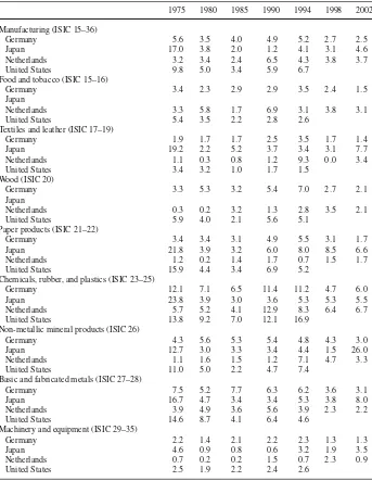
used to report abatement capital expenditures and the ISIC (Rev. 3) system.8Table1reports

the percent of capital expenditures assigned to abatement activities for selected years. Aside from sampling error, fluctuations in the share of capital expenditures assigned to pollution abatement can be explained by whether new regulations are being implemented.

FollowingHarrigan(1999), theOECD STructural ANalysis (STAN) Database for

Indus-trial Analysis, which provides industry-level data for Organization for Economic Cooperation and Development (OECD) countries from 1970 to the present, is our primary source of

capi-tal expenditure data.9_{The product of the share of capital expenditures assigned to abatement}

activities and gross private fixed capital formation in current prices (GFCF) yields our esti-mate of capital expenditures assigned to abatement activities. Subtracting abatement capital expenditures from GFCF yields capital expenditures assigned to good output production.

Because the STAN Database does not provide capital stock estimates, we adopt the

per-petual inventory method employed byHarrigan(1999) and use GFCF and the index of gross

capital fixed formation (GFCFK) to derive real capital expenditures,i. Assuming capital has

a useful life of 10 years (T=10) and an annual depreciation rate of 15% (δ=0.15), allows

us to derive the real capital stock for industryjin countrycfor yeart:

kcj t = T

n=1

(1−δ)n−1icj,t−n

In this distributed lag specification, the capital stock assigned to good output production

and pollution abatement in periodt consists of capital expenditures from periodt−1 to

periodt−10.10

TheGroningen Growth and Development Centre(2006) is our source for total annual hours worked, which is our measure of labor. Finally, we use value added in current prices

8_{The industry concordances developed by}_Bouman₍₁₉₉₈_{, p. 22) are the starting point for our concordances} for Germany, the Netherlands, and the United States. We developed the concordance for industries in Japan. All concordances are discussed in the Supplementary material. All GAMS programs, data, and the Supplementary material are available from the corresponding author upon request.

9_{We employ data downloaded from the OECD STAN database in October 2004 and June 2005. Data in the} STAN database are classified with ISIC, Rev. 3 codes. The Supplementary material explains how we derived values the non-metallic minerals (ISIC 26) industry in the Netherlands. Because the downloaded OECD data contained no capital expenditure data for Japan, we used theOECD STAN Database for Industrial Analysis, 1974–1993 (OECD 1995)and theOECD STAN Database for Industrial Analysis, 1978–1997(OECD 1999) to develop a consistent set of capital expenditure estimates for 1973–1994. We then use changes in 1994– 2003 capital expenditure values in theJapan Statistical Yearbook(Japan, 1997–2005), to extrapolate the 1994 OECD values to 1995–2002.

(9)

Table 1 Percent of capital expenditures assigned to air, water, and solid waste pollution abatement 1975 1980 1985 1990 1994 1998 2002 Manufacturing (ISIC 15–36)

Germany 5.6 3.5 4.0 4.9 5.2 2.7 2.5

Japan 17.0 3.8 2.0 1.2 4.1 3.1 4.6

Netherlands 3.2 3.4 2.4 6.5 4.3 3.8 3.7

United States 9.8 5.0 3.4 5.9 6.7

Food and tobacco (ISIC 15–16)

Germany 3.4 2.3 2.9 2.9 3.5 2.4 1.5

Japan

Netherlands 3.3 5.8 1.7 6.9 3.1 3.8 3.1

United States 5.4 3.5 2.2 2.8 2.6

Textiles and leather (ISIC 17–19)

Germany 1.9 1.7 1.7 2.5 3.5 1.7 1.4

Japan 19.2 2.2 5.2 3.7 3.4 3.1 7.7

Netherlands 1.1 0.3 0.8 1.2 9.3 0.0 3.4

United States 3.4 3.2 1.0 1.7 1.5

Wood (ISIC 20)

Germany 3.3 5.3 3.2 5.4 7.0 2.7 2.1

Japan

Netherlands 0.3 0.2 3.2 1.3 2.8 3.5 2.1

United States 5.9 4.0 2.1 5.6 5.1

Paper products (ISIC 21–22)

Germany 3.4 3.4 3.1 4.9 5.5 3.1 1.7

Japan 21.8 3.9 3.2 6.0 8.0 8.5 6.6

Netherlands 1.2 0.2 1.4 1.7 0.7 1.5 1.7

United States 15.9 4.4 3.4 6.9 5.2

Chemicals, rubber, and plastics (ISIC 23–25)

Germany 12.1 7.1 6.5 11.4 11.2 4.7 6.0

Japan 23.8 3.9 3.0 3.6 5.3 5.3 5.5

Netherlands 5.7 5.2 4.1 12.9 8.3 6.4 6.7

United States 13.8 9.2 7.0 12.1 16.9

Non-metallic mineral products (ISIC 26)

Germany 4.3 5.6 5.3 5.4 4.8 4.3 3.0

Japan 12.7 3.0 3.3 3.4 4.4 1.5 26.0

Netherlands 1.1 1.6 1.5 1.2 7.1 4.7 3.3

United States 11.0 5.0 2.2 4.7 7.4

Basic and fabricated metals (ISIC 27–28)

Germany 7.5 5.2 7.7 6.3 6.2 3.6 3.1

Japan 16.7 4.7 3.4 3.4 5.3 3.8 8.0

Netherlands 3.9 4.9 3.6 5.6 3.9 2.3 2.2

United States 14.6 8.7 4.1 6.4 4.6

Machinery and equipment (ISIC 29–35)

Germany 2.2 1.4 2.1 2.2 2.3 1.3 1.3

Japan 4.6 0.9 0.8 0.6 3.2 1.9 3.5

Netherlands 0.7 0.2 0.2 1.5 0.7 2.3 0.9

United States 2.5 1.9 2.2 2.4 2.6

(VALU) and the index of value added (VALUK) from the OECD STAN Database to derive real value added.

(10)

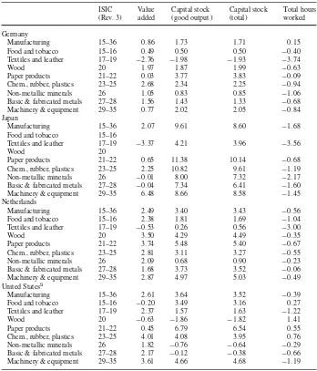
Table 2 Summary statistics: Average annual percent growth of inputs and output (1985–2002)

ISIC Value Capital stock Capital stock Total hours (Rev. 3) added (good output ) (total) worked Germany

Manufacturing 15–36 0.86 1.73 1.71 0.15

Food and tobacco 15–16 0.49 0.50 0.50 −0.40

Textiles and leather 17–19 −2.76 −1.98 −1.93 −3.74

Wood 20 1.97 1.87 1.99 −0.63

Paper products 21–22 0.03 3.77 3.83 −0.09

Chem., rubber, plastics 23–25 2.68 2.34 2.25 −0.94

Non-metallic minerals 26 1.05 0.83 0.85 −1.06

Basic & fabricated metals 27–28 1.56 1.43 1.33 −0.68

Machinery & equipment 29–35 0.77 2.02 2.05 −0.84

Japan

Manufacturing 15–36 2.07 9.61 8.60 −1.68

Food and tobacco 15–16

Textiles and leather 17–19 −3.37 4.21 3.96 −3.56

Wood 20

Paper products 21–22 0.65 11.38 10.14 −0.68

Non-metallic minerals 26 −0.01 8.00 7.32 −2.17

Basic & fabricated metals 27–28 −0.04 7.34 6.41 −1.60

Netherlands

Manufacturing 15–36 2.49 3.40 3.43 −0.56

Food and tobacco 15–16 2.38 1.81 1.69 −1.04

Textiles and leather 17–19 −0.53 0.26 0.56 −3.00

Wood 20 3.50 4.29 4.49 −0.35

Paper products 21–22 3.74 5.48 5.40 −0.67

Non-metallic minerals 26 2.09 0.68 0.90 −0.23

Basic & fabricated metals 27–28 1.68 3.73 3.52 −0.06

United Statesa

Manufacturing 15–36 2.61 3.64 3.52 −0.39

Food and tobacco 15–16 −0.20 3.49 3.16 0.27

Textiles and leather 17–19 2.37 1.57 1.63 −1.22

Wood 20 −0.63 −1.86 −1.82 1.41

Paper products 21–22 0.45 6.79 6.54 0.55

Chem., rubber, plastics 23–25 4.01 4.08 3.95 0.76

Non-metallic minerals 26 1.82 −0.76 −0.64 −0.29

Basic & fabricated metals 27–28 2.17 −0.12 −0.38 −0.66

a_{United States annual changes are for 1985–1994}

Value added for each industry in domestic currencies (i.e., Euros and yen) is multiplied by its

respective 1997 UVR. LikeHarrigan(1999), the Penn World Table (PWT) Version 6.2 (see

Heston et al. 2006) is our source of purchasing power parity data for investment expenditures. Therefore, we convert investment expenditures to U.S. dollars using a single PPP for each country for each year.

Table2presents summary statistics of growth rates of value added, employment, and

(11)

We calculate our meta-frontiers using a windows technology.11For example, the

produc-tion technology of periodt+1 consists of observations from periodst+1,t, andt−1, while

the production technology of periodtconsists of observations from periodst,t−1, andt−2.

For each 2-year pair, four LP problems are solved for both the regulated and unregulated technologies. Because we use “windows” to model the production technology, our sample generates results for 2-year pairs starting in 1986–1987 and continuing through 1992–1993 for the United States, and 2000–2001 for Germany, Japan, and the Netherlands.

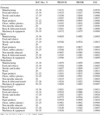
Table3presents the geometric means of annual changes in PRODUR, PRODR, and PAI

for the manufacturing sector and its associated industries.12While the manufacturing sector

of United States with a PAI of 1.0011 is most adversely affected by pollution abatement, regulated productivity growth in the manufacturing sector of Germany is higher than

unreg-ulated productivity growth (PAI=0.9976). In addition, it can be seen that there is substantial

variation across industries. For the food industry (ISIC 15–16), the PAI ranges from 0.9998 for Germany to 1.0045 for the Netherlands. For the textile industry (ISIC 17–19), the range of the PAI is from 1.0000 for Germany to 1.0037 for the Netherlands. For the wood industry (ISIC 20), PAI ranges from 0.9991 for the United States to 1.0037 for Germany. For the paper industry (ISIC 21–22), the range of PAI is from 1.0000 for Germany to 1.0085 for Japan. For the chemical industry (ISIC 23–25), the PAI ranges from 0.9989 for the Netherlands to 1.0016 for Japan. For the non-metals mineral industry (ISIC 26), the range of PAI is from 0.9984 for the United States to 1.0044 for Japan. For the basic and fabricated metals industry (ISIC 27–28), the PAI ranges from 0.9994 for the Netherlands to 1.0007 for the United States. For the machinery and equipment industry (ISIC 29–35), the range of PAI is from 0.9997 for the Netherlands to 1.0009 for Japan. Overall, the largest decline in productivity change associated with pollution abatement involves the paper industry of Japan, while the largest increase in productivity associated with pollution abatement involves the non-metallic min-erals industry in the United States. While it is difficult to make causality statements about observed changes in productivity, the PAI values indicate assigning capital expenditures to pollution abatement did not have a substantial affect on productivity growth. In addition, our results reveal the importance of assessing the effect of pollution abatement using industry instead of economy-wide data on pollution abatement costs. For example, during the 1987– 2001 period Germany has a low PAI for the entire manufacturing sector, while it has a high PAI for the wood (ISIC 20) industry. Finally, out results indicate substantial variation in productivity effects across time periods.

For industries where PRODR and PAI assume values greater than unity (e.g., the non-metallic minerals industry in Germany), increased rates of productivity growth occurred simultaneously with increased levels of pollution abatement. In addition, industries where PRODR and PAI are less than unity (e.g., the chemical industry of the United States) simulta-neously experienced decreased rates of productivity growth with decreased levels of pollution abatement. For industries where PRODR exceeds unity while PAI is less than unity (e.g., the chemical industry in the Netherlands), increased productivity growth is associated with decreased levels of pollution abatement. Finally, PRODR less than unity and PAI greater than unity (e.g., the paper industry in Japan), signifies a case where decreased productivity growth is associated with increased levels of pollution abatement.

11_Shestalova₍₂₀₀₃_{) compared changes in productivity and efficiency calculated using DEA with} contempo-raneous and sequential frontiers, whileAsmild et al.(2004) investigated the consequences of using ‘windows’ instead of contemporaneous frontiers.

(12)

Table 3 Pollution abatement index, 1987–2001 (geometric means of 2-year pair values)

ISIC (Rev. 3) PRODUR PRODR PAI

Germany

Manufacturing 15–36 1.0131 1.0156 0.9976

Food and tobacco 15–16 1.0125 1.0127 0.9998

Textiles and leather 17–19 1.0240 1.0240 1.0000

Wood 20 1.0247 1.0209 1.0037

Paper products 21–22 0.9993 0.9993 1.0000

Chem., rubber, plastics 23–25 1.0191 1.0191 1.0000

Non-metallic minerals 26 1.0194 1.0157 1.0036

Basic & fabricated metals 27–28 1.0261 1.0261 1.0000

Machinery & equipment 29–35 1.0172 1.0175 0.9998

Japan

Manufacturing 15–36 0.9855 0.9852 1.0003

Food and tobacco 15–16

Wood 20

Paper products 21–22 0.9911 0.9827 1.0085

Netherlands

Manufacturing 15–36 1.0079 1.0078 1.0000

Food and tobacco 15–16 1.0344 1.0298 1.0045

Wood 20 1.0211 1.0200 1.0011

Paper products 21–22 1.0241 1.0232 1.0008

United Statesa

Manufacturing 15–36 1.0021 1.0010 1.0011

Food and tobacco 15–16 0.9910 0.9896 1.0014

Wood 20 0.9775 0.9784 0.9991

Paper products 21–22 0.9918 0.9909 1.0010

a_{Results for United States are for 1987–1993}

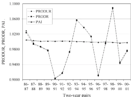
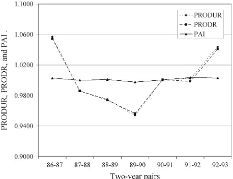
In order to view variations in annual changes that are obscured by the averages reported

in Table3, we plot PRODUR, PRODR, and PAI for the manufacturing sectors of Germany,

Japan, the Netherlands, and the United States in Figs.1,2,3and4. Viewing these figures

(13)

Fig. 1 Trends in PRODUR, PRODR, and PAI for manufacturing in Germany (1987–2001)

Fig. 2 Trends in PRODUR, PRODR, and PAI for manufacturing in Japan (1987–2001)

of the manufacturing sectors of Germany (1.0081) and Japan (1.0021) are much higher

than those reported in Table3 for 1987–2001. As a result, only the PAI of the

(14)

Fig. 3 Trends in PRODUR, PRODR, and PAI for manufacturing in the Netherlands (1987–2001)

Fig. 4 Trends in PRODUR, PRODR, and PAI for manufacturing in the United States (1987–1993)

(15)

5 Conclusions

We investigated the association between pollution abatement capital expenditures and pro-ductivity growth for manufacturing industries in Germany, Japan, the Netherlands, and the United States from the 1987 through 2001. We believe this study represents the first appli-cation of pollution abatement capital expenditure data from these four countries being used in the same study.

Because releasing capital from pollution abatement results in the unregulated technology producing more of the good output than the regulated technology, the traditional view is that pollution abatement is associated with reduced rates of productivity growth. In our study, PAI measures productivity changes associated with assigning capital to pollution abatement. The primary finding of our study is that since the mid-1980s there are relatively small dif-ferences in productivity growth for the regulated and unregulated technologies. In our model, this can be seen in PAI values close to unity. This is the consequence of similar growth rates for capital stock assigned to good output production and capital stock assigned to pollution abatement. If data existed back to the onset of assigning capital expenditures to pollution abatement, we suspect more substantial differences between PRODUR and PRODR would be observed. As a result of this evidence, our primary conclusion is pollution abatement capital expenditures are not associated with a substantial decline in manufacturing productivity.

As was the case for previous cross-country productivity studies, we confronted several problems in the course of developing data for our meta-frontier analysis. One problem is the reunification of Germany and the conversion of data from West Germany to the

re-uni-fied Germany.13In addition, the most recent STAN databases do not provide gross capital

formation data for Japan. This forced us to use different sources for the capital expenditure estimates for Japan. Finally, the standard caveats associated with converting value added and gross capital formation data to U.S. dollars are compounded by the conversion of pre-Euro value added and capital formation data for Germany and the Netherlands into Euros via their

January 1, 1999 irrevocable conversion rates (seeSchreyer and Suyker 2002, p. 7).

Both the model we specified and the data employed to implement it assume assigning capital expenditures to either good output production or pollution abatement is a feasible undertaking. Although widely used, several concerns have been raised about these surveys (seeBecker and Shadbegian 2007;Gallaher et al. 2008). The primary concern involves the dif-ficulty associated with estimating “change in production process” capital expenditures (e.g., convert plant to consume fuels that generate fewer emissions). As the share of pollution abatement capital expenditures associated with change-in-process techniques increases— and the relative importance of end-of-pipe abatement expenditures declines—it becomes increasingly difficult to determine which capital expenditures are associated with abatement

activities.14In spite of these concerns, survey estimates of pollution abatement capital

expen-ditures remain the best data currently available to compare changes in the absolute and relative burden of abatement costs incurred by the four countries in our sample.

Information on air and water pollution abatement capital expenditures assigned to change-in-process (CIP) and end-of-pipe (EOP) abatement strategies in Germany and the United

13_{The 1995 issue (p. 704) of}_{Statistisches Jahrbuch}₍_{Federal Republic of Germany}_{) reports shares of capital} expenditures assigned to pollution abatement by manufacturing and non-manufacturing plants in the former West Germany of 5.0 and 4.8% for 1991 and 1992, respectively. Comparable values for the unified Germany were 5.3 and 5.6%.

(16)

States provides some additional insights. The share of pollution abatement capital expendi-tures categorized as CIP expendiexpendi-tures increased from 15.5% in 1973 to 41.7 in 1994 (i.e., a 170% share increase) for the USA. Interestingly, the 2003 CIP share for the manufacturing sector in Germany was only 32%. There is substantial variation both in trends and shares for the last year for which data are available. Among pollution-intensive industries in Germany, only the chemical industry (ISIC 24) has an above average share of pollution abatement capital expenditures categorized as CIP. On the other hand, petroleum refining (ISIC 23) and rubber and plastics (ISIC 25) both report below average shares. For the USA, petroleum (ISIC 23) and chemicals (ISIC 24) report above average shares in 1994, while rubber and plastics (ISIC 25) report below average shares. While the share of pollution abatement capital expenditures categorized as CIP exhibits a substantial increase in USA manufacturing, there is substantial variation across industries. For example, petroleum and coal products (ISIC 23) and fabricated metals (ISIC 28) report share increases of 350% in CIP abatement techniques between 1973 and 1994, while non-metallic minerals (ISIC 26) increased only 50%, wood (ISIC 20) increased 70%, and primary metals (ISIC 27) increased 80%.

Our inability to account for employment and intermediate inputs—such as energy— assigned to pollution abatement represents a shortcoming of the empirical analysis presented in this study. A review of trends in the ratio of annual pollution abatement current account costs for air, water, and solid waste abatement to industry output reveals this ratio doubled

between 1973 and 1994 for USA manufacturing (U.S. Department of Commerce, 1978–

1996). Interestingly, more pollution intensive-industries experienced smaller than average

in-creases, while less pollution-intensive industries experienced higher than average increases. Although this ratio increased by 50% between 1984 and 2003 for manufacturing in the Netherlands, the 2003 ratio for the Netherlands, it is still less than the 1994 USA value. Finally, while this ratio decreased by 20% between 1996 and 2002 for manufacturing in Germany, its 2002 value is higher than the 1994 USA value.

While it is difficult to make an exact assessment of the bias introduced by using only capital expenditure data, a simple assessment would be this approach introduces no biases if other inputs are assigned to pollution abatement in the same proportion as capital. It follows that our results understate the association between pollution abatement and productivity if the share of other inputs assigned to pollution abatement is higher than the share for capital; while our results overstate the association between pollution abatement and productivity if the share of other inputs assigned to pollution abatement is less than the share for capital. One approach to determine the importance of this exclusion involves using Bureau of the Census of the United States (1973–1994) data on labor and material, supplies, services, and equipment leasing costs assigned to pollution abatement. This would permit a comparison of our “capital stock only” results with results that calculate the association between abatement activities and productivity for U.S. manufacturing industries using the data on capital, labor, and aggregate intermediate inputs assigned to pollution abatement.

Finally, it would be useful to undertake a more thorough investigation of the associa-tion between the assigned input and joint producassocia-tion models. This investigaassocia-tion involves modeling a network technology that requires information not only on good and bad output production, but also data on inputs assigned to good output production and inputs assigned to abatement activities. This would permit an investigation into discrepancies in the productivity results produced by the joint production and assigned input models, and the consequences of adopting EOP and CIP abatement strategies.

(17)

Schäfer, Carsten Stahmer, and Kimio Uno for assistance with the pollution abatement expenditure data. Some of the research for this paper was conducted at the Library of Congress and was facilitated by the staff of the Asian Reading Room.

References

Asmild M, Paradi JC, Aggarwall V, Schaffnit-Chatterjee C (2004) Combining dea window analysis with the malmquist index approach in a study of the canadian banking industry. J Product Anal 21(1):67–89 Becker RA, Shadbegian RJ (2007) Issues and challenges in measuring environmental expenditures by U.S.

manufacturing: the redevelopment of the pace survey. Working paper 07-20, Center for Economic Stud-ies, U.S. Census Bureau or Working Paper no. 2007-08, National Center for Environmental Economics, U.S. Environmental Protection Agency

Bouman M (1998) Environmental costs and capital flight. Tinbergen Institute Research Series, vol 177. Thesis Publishers, Amsterdam

Caves DW, Christensen LR, Diewert WE (1982) The economic theory of index numbers and the measurement of input, output, and productivity. Econometrica 50(6):1393–1414

Conrad K, Morrison C (1989) The impact of pollution abatement investment on productivity change: an empirical comparison of the U.S., Germany, and Canada. South Econ J 55(3):684–698

Conrad K, Wastl D (1995) The impact of environmental regulation on productivity in german industries. Empir Econ 20(4):615–633

Denison EF (1978) Effects of selected changes in the institutional and human environment upon output per unit of input. Surv Curr Bus 58(1):21–44

Färe R, Grosskopf S, Norris M et al (1994) Productivity growth, technical progress and efficiency change in industrialized countries. Am Econ Rev 84(1):66–83

Färe R, Grosskopf S, Pasurka C (2007) Pollution abatement activities and traditional productivity. Ecol Econ 62(3–4):673–682

Federal Republic of Germany, Statistiche Bundesamt (1978–2003) Statistisches jahrbuch. Wiesbaden Federal Republic of Germany, Statistiche Bundesamt (1980,2000,2004–2005), Investitionen für umweltschutz

im produzierenden gewerbe, Unwelt, Fachserie 19, Reihe 3, Wiesbaden

Gallaher M, Morgan C, Shadbegian R (2008) Redesign of the 2005 pollution abatement costs and expenditure survey. Working paper no. 2008-01, National Center for Environmental Economics, U.S. Environmental Protection Agency

Gray WB, Shadbegian RJ (2003) Plant vintage, technology, and environmental regulation. J Environ Econ Manag 46(3):384–402

Groningen Growth and Development Centre, ICOP Database 1997 Benchmark.http://www.ggdc.net

Groningen Growth and Development Centre (2006) 60-Industry database. September.http://www.ggdc.net

Harrigan J (1999) Estimation of cross-country differences in industry production functions. J Int Econ 47(2):267–293

Heston A, Summers R, Aten B (2006), Penn world table version 6.2, center for international comparisons at the University of Pennsylvania, September.http://pwt.econ.upenn.edu/php_site/pwt_index.php

Inklaar R, Wu H, van Ark B (2003) ‘Losing ground’ Japanese labour productivity and unit labour costs in manufacturing in comparison to the U.S. Research Memorandum GD-64, Groningen Growth and Development Centre, University of Groningen

Jaffe AB, Peterson SR, Portney PR, et al (1995) Environmental regulation and the competitiveness of U.S. manufacturing: what does the evidence tell us? J Econ Lit 33(1), 132–163

Japan (1997–2005), Japan statistical yearbook

Lau LJ, Yotopoulos PA (1989) The meta-production function approach to technological change in world agriculture. J Dev Econ 31(2):241–269

Millimet DL, Osang T (2003) Environmental regulation and productivity growth: an analysis of US manu-facturing industries. In: Böehringer C, Löeschel A (eds) Empirical modeling of the economy and the environment. ZEW economic studies, vol 20. Physica Verlag, Heidelberg, pp 7–22

Ministry of Economy, Trade, and Industry, Japan (2002–2004) Survey results of investments for industrial pollution control facilities

Ministry of International Trade and Industry, Japan (1977–2001) Survey results of investments for industrial pollution control facilities. In Plant and equipment investment plans in major industries (Shuy¯o Sangy¯o no Setsubi T¯oshi Keikaku), Ministry of finance printing bureau, Tokyo

(18)

OECD, Economic analysis and statistics division (1995,1999) The oecd stan database for industrial analysis. OECD, Paris

Pasurka C (2008) Perspectives on pollution abatement and competitiveness: theory, data, and analyses. Rev Environ Econ Policy 2(2):194–218

Pyrwes M (1984) The cost in lost productivity of new regulation in the U.S. chemical industry. J Policy Model 6(3):411–419

Schreyer P, Suyker W (2002) Creation of the euro area: implications for economic statistics. OECD Statistics Brief, February, No. 2

Shadbegian RJ, Gray WB (2006) Assessing multi-dimensional performance: environmental and economic outcomes. J Product Anal 26(4):213–234

Shephard RW (1970) Theory of cost and production functions. Princeton University Press, Princeton, NJ Shestalova V (2003) Sequential malmquist indices of productivity growth: an application to oecd industrial

activities. J Product Anal 19(2–3):211–226

Uno K (1987) Pollution prevention and environmental quality. In: Japanese industrial performance, Chapter 16. North Holland, New York, pp 271–310

Uno K (1995) Pollution prevention investment. In: Environmental options: accounting for sustainability. Economy & environment, vol 10, Chapter 6. North Holland, New York, pp 143–198

U.S. Congress, Congressional Budget Office (1985) Environmental regulation and economic efficiency. US Government Printing Office, Washington, DC

U.S. Department of Commerce, Bureau of the Census (1978–1996) Pollution abatement costs and expendi-tures. Current Industrial Reports, MA200. U.S. Government Printing Office, Washington, DC.http:// www.census.gov/prod/2/manmin/ma200x94.pdf

Valentini L (2003) Pollution abatement expenditures and international competitiveness: estimation of to-tal factor productivity. Paper presented at the 12th annual conference of the european association of environmental and resource economists, Bilbao, Spain, 28–30 June 2003

(19)