Numerical modeling, Finite difference method; Finite element method method; Finite element method, Computer models

(1)

M odu le 4 – ( L1 2 - L1 8 ) : “

W a t e r sh e d M ode lin g”

St a n da r d m ode lin g a ppr oa ch e s a n d cla ssifica t ion s, syst e m con ce pt St a n da r d m ode lin g a ppr oa ch e s a n d cla ssifica t ion s, syst e m con ce pt for w a t e r sh e d m ode lin g, ove r a ll de scr ipt ion of diffe r e n t h ydr ologic pr oce sse s, m ode lin g of r a in fa ll, r u n off pr oce ss, su bsu r fa ce flow s a n d gr ou n dw a t e r flowg

1 7

N u m e r ica l W a t e r sh e d

1 1 1

(2)

L1 7

L1 7 –

N u m e r ica l W a t e r sh e d

M d li

M ode lin g



Topics Cove r e d



Topics Cove r e d



Physically based wat ershed m odeling,

Num erical m odeling, Finit e difference

m et hod; Finit e elem ent m et hod

m et hod; Finit e elem ent m et hod,

Com put er m odels



(3)

W a t e r sh e d M ode lin g

• Transform at ion of rainfall int o runoff over a wat ershed • Generat ion of flow hydrograph for t he out let

• Generat ion of flow hydrograph for t he out let

• Use of t he hydrograph at t he upst ream end t o rout e t o t he downst ream end

H d l i i l t i d l t h t i l t i

• Hydrologic sim ulat ion m odels use m at hem at ical equat ions t o calculat e result s like runoff volum e or peak flow

• Com put er m odels allows param et er variat ion in space and p p p t im e – w it h use of num erical m et hods

• Ease in sim ulat ion of com plex rainfall pat t erns and het erogeneous wat ersheds

12.00

het erogeneous wat ersheds

3 3

(4)

H ydr ologic M ode ls

y

g

Model Type

Example of Model

Lumped Parameter

p

Synder Unit Hydrograph

y

g

p

Distributed Kinematic

wave

Event

HEC-1, SWMM

Event

HEC 1, SWMM

Continuous

Stanford Watershed Model,

SWMM, HSPF,

,

Physically based

HEC-1, SWMM, HSPF

Stochastic

Synthetic stream flows

Stochastic

Synthetic stream flows

Numerical

Explicit kinematic wave

Analytical

Nash IUH

(5)

 Flow of wat er in a wat ershed is a dist ribut ed process

N e ce ssit y of D ist r ibu t e d m ode ls

 Flow of wat er in a wat ershed is a dist ribut ed process  Models should be physically based

 Governing equat ions – St . Venant equat ions g q q

 Com put er m odels- based on t he St . Venant equat ions

 Allows com put at ion of flow rat e and wat er level as funct ions

f d t i of space and t im e

 Model m ore closely approxim at es t he act ual unst eady

non-uniform nat ure of flow propagat ion in channels p p g

Rainf Rainf all

I filt ti

Channel flow

5 5

Infiltration

(6)

H ydr ologic/ H ydr a u lic M ode lin g

 Hydrological / Hydraulic m odel- concept ual or

physically based procedure- num erically solving hydrological processes - diagnose or forecast hydrological processes diagnose or forecast processes.

 Physical based: descript ion of nat ural syst em using

basic m at hem at ical represent at ion of flows of m ass basic m at hem at ical represent at ion of flows of m ass, m om ent um and various form s of energy.

 Dist ribut ed: consider spat ial variat ion of variables &

param et ers.

 Applicat ions: Rainfall t o runoff , Surface wat er/

groundwat er assessm ent Flood/ drought predict ions groundwat er assessm ent , Flood/ drought predict ions, Evaluat ion of wat ershed / cat chm ent m anagem ent st rat egies, River basin / Agricult ural wat er

(7)

(8)

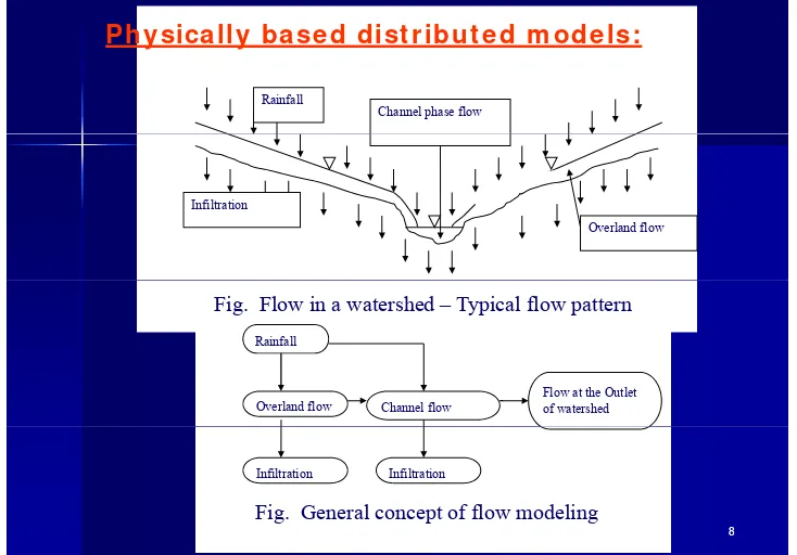
Ph ysica lly ba se d dist r ibu t e d m ode ls:

Rainfall

Channel phase flow

Infiltration Infiltration

Overland flow

Rainfall

Fig. Flow in a watershed – Typical flow pattern

Flow at the Outlet of watershed Channel flow

Overland flow

Infiltration Infiltration

(9)

Ph ysica lly

Ph ysica lly Ba se dBa se d M ode lM ode l –– Ove r la n dOve r la n d FlowFlow Equ a t ion s

Equ a t ion s Equ a t ion s Equ a t ion s

Con t in u it y

Con t in u it y e qu a t ione qu a t ion

M om e n t u m

M om e n t u m Equ a t ionEqu a t ion

I n it ia l a n d Bou n da r y con dit ion sy

I C for overland is usually of dry bed condit ion. At t im e t = 0, h = 0 and q = 0 at all nodal point s

Upst ream boundary condit ion is assum ed as zero

9 9

inflow s; h = 0 and q = 0 at all t im es

(10)

Gov. Equat ion for Channel Flow

(11)

Solut ion Met hodologies

 An a lyt ica l m e t h od: For t he given m at hem at ical

form ulat ion, an analyt ical expression involving t he

param et ers and t he independent variables are obt ained using various m at hem at ical procedures.

 Main lim it at ion- only for a sm all class of m at hem at ical

form ulat ions w it h sim plified governing equat ions, boundary condit ions & geom et ry, analyt ical solut ions can be obt ained.

 Ph ysica l m e t h od: As t he m at hem at ical m odel represent s a

real physical syst em , alt hough on cert ain idealized p y y , g

assum pt ions, variables and param et ers of t he m odel can be considered as having physical dim ensions and can be

analyzed som et im es in t he laborat ory or in t he field it self.

 The physical m odels are used less frequent ly since it is

expensive, cum bersom e and difficult in pract ice.

 Com pu t a t ion a l m e t h od

11 11

(12)

Com put at ional Met hod



I n t he com put at ional m et hod, t he solut ion is

obt ained w it h t he help of som e approxim at e

m et hods using a com put er. Com m only,

num erical m et hods are used t o obt ain solut ion

i t h

t t i

l

t h d

in t he com put at ional m et hod.

Wid

l

f

t h

t i

l f

l t i

&



Wider class of m at hem at ical form ulat ions &

advent of fast com put ers, com put at ional

m odels have becom e t he m ost widely used

valuable t ool for solving t he engineering

(13)

Num erical Modeling



Variet y of num erical m et hods such

as

- M e t h od of ch a r a ct e r ist ics

- Fin it e D iffe r e n ce M e t h od ( FD M )

i i

l

h d (

)

- Fin it e V olu m e M e t h od ( FV M )

- Fin it e Ele m e n t M e t h od ( FEM )

- Bou n da r y Ele m e n t M e t h od ( BEM )

.

13 13

(14)

Finit e Difference Met hod

C i i i f h f i d b

 Cont inuous variat ion of t he funct ion concerned by a set

of values at point s on a grid of int ersect ing lines.

 The gradient of t he funct ion are t hen represent ed by e g ad e o e u c o a e e ep ese ed by differences in t he values at neighboring point s and a finit e difference version of t he equat ion is form ed.

 At point s in t he int erior of t he grid t his equat ion is used  At point s in t he int erior of t he grid, t his equat ion is used

t o form a set of sim ult aneous equat ions giving t he value of t he funct ion at a point in t erm s of values at nearby

i t point s.

 At t he edges of t he grid, t he value of t he funct ion is

(15)

Met hod of charact erist ics ( MOC)

MOC d i l diff i l i f il

 MOC - reduce a part ial different ial equat ion t o a fam ily

of ordinary different ial equat ions along which t he

solut ion can be int egrat ed from som e init ial dat a given on a suit able hyper surface

 For a first - order PDE, MOC discovers curves ( called

charact erist ic curves or charact erist ics) along which PDE charact erist ic curves or charact erist ics) along which PDE becom es an ODE. I t is solved along t he charact erist ic curves & t ransform ed int o a solut ion for original PDE. V i t f FDM it bl f l i h b li

 Variant of FDM – suit able for solving hyperbolic

equat ions

 MOC t o sim ulat e advect ion dom inat ed t ransportp  Track idealized part icles t hrough flow field

 Efficient & m inim ize num erical inst abilit ies

15 15

(16)

Finit e Elem ent Met hod

 The region of int erest is divided in a m uch m ore

flexible way flexible way

 The nodes at which t he value of t he funct ion is found

have t o lie on a grid syst em or on a flexible m esh

h b d d h dl d

 The boundary condit ions are handled in a m ore

convenient m anner.

 Direct approach, variat ional principle or weight ed Direct approach, variat ional principle or weight ed

(17)

Boundary Elem ent Met hod

 The part ial different ial equat ions describing t he

dom ain, is t ransform ed in t o an int egral equat ion dom ain, is t ransform ed in t o an int egral equat ion relat ing only t o boundary values.

 The m et hod is based on Green’s int egral t heorem .

h b d d d d f h d

 The boundary is discret ized inst ead of t he dom ain.  A 3- Dim ensional problem reduces t o a

2- Dim ensional problem and 2- Dim ensional problem in 2 Dim ensional problem and 2 Dim ensional problem in t o 1- Dim ensional problem .

 BEM is ideally suit ed t o t he solut ion of m any t wo and

h di i l bl i l i i d i l t hree- dim ensional problem s in elast icit y and pot ent ial t heory

(18)

Analyt ical Solut ion–Kinem at ic wave

f

S_f

o

S

n

 

5 



• Analyt ical solut ion for one- dim ensional kinem at ic

3 



wave equat ions is given by above equat ions ( Jaber and Moht ar, 2003) ; t_c is t im e of concent rat ion ( sec) ; t_r is

rainfall durat ion ( sec) ; t_f is t he sim ulat ion t im e ( sec) ;

Lw is t he lengt h of wat ershed ( m ) in t he direct ion of m ain slope. ( Jaber, F.H., and Moht ar, R.H. ( 2003) . “ St abilit y and accuracy of t wo dim ensional kinem at ic

l d fl d li ” Ad i W t

(19)

Fin it e D iffe r e n ce M e t h od ( FD M )

 FD M : Calculat ions are perform ed on a grid placed

over t he ( x, t ) plane

 Flow and wat er surface elevat ion are obt ained for  Flow and wat er surface elevat ion are obt ained for increm ent al t im e and dist ances along t he channel

 Ex plicit m e t h ods: calculat es values of velocit y &

d h d b d l k

dept h over a grid syst em based on a previously known dat a for t he river reach

 I m plicit m e t h ods:I m plicit m e t h ods: set up a series of sim ult aneousset up a series of sim ult aneous

num erical equat ions over a grid syst em for t he ent ire river & equat ions are solved at each t im e st ep.

Fig: x - t pla n e for fin it e diffe r e n ce sch e m e

19 19

(20)

Typical St eps for FDM m odel

– Governing Part ial

Different ial Equat ions wit h Subsidiary condit ions

Subsidiary condit ions

– Divide dom ain int o Grids – Transform at ion by Finit e y

Difference Met hod – Syst em of difference

equat ions equat ions

– Applicat ion of Boundary Condit ions

I,J+1

Δ

y

I-1 J

I J

I+1 J

– Solve by direct or it erat ive

m et hod – Solut ion

Δ

y

I 1,J

I,J

I+1,J

Δ

x

I,J-1

(21)

Finit e Difference Schem e

There are t hree com m only used finit e difference approxim at ions finit e difference approxim at ions for t he solut ion of PDE

b) Forward difference schem e c) Cent ral difference schem e

1

(22)

i-1, j+1 i-1, j+1 i+1, j+1

∆t

i j

i 1 j i+1 j

Finit e Difference

Schem e

∆x ∆x

i, j

i-1, j i+1, j

Cross-sectional view in x-t plane

h0, Q0, t1 h1, Q1, t1 h2, Q2, t2 x-t plane

p

0, 0, 1 1, 1, 1 2, 2, 2

∆t _h

0, Q0, t0 h1, Q1, t0 h2, Q2, t0

(23)

Fin it e D iffe r e n ce Appr ox im a t ion s

Tem poral derivat ive

t

Spat ial derivat ive

x

Spat ial derivat ive is writ t en using t erm s on know n t im e line

Spat ial and t em poral

derivat ives use unknow n t im e lines for com put at ion

23 23

t erm s on know n t im e line _{lines for com put at ion}

(24)

Fin it e Ele m e n t M e t h od

 1D- Kinem at ic & Diffusion Wave Models for Overland Flow  One- dim ensional m odel wit h linear line elem ent s

 One- dim ensional m odel wit h linear line elem ent s  Apply Galerkin FEM for 1D cont inuit y equat ion

 - - - ( 1)

( 2)

 - - - ( 2)

 Expansion of Eq considering it for one elem ent is given as  Expansion of Eq considering it for one elem ent is given as

(25)

Fin it e Ele m e n t M e t h od

 Shape funct ion N for a linear elem ent can be expressed as [ N] =

[ N1 N2] Where N_i = 1- ( x/ L) and N_j = x/ L

E t i b it t i t i f f ll

Fin it e Ele m e n t M e t h od

 Equat ion can be w rit t en in m at rix form as follows:



( 4) - - - ( 4)

 Assem bling t he overland flow line elem ent s and applying im plicit

finit e difference schem e for t im e dom ain

 - - - ( 5)

25 25

(26)

Fin it e Ele m e n t M e t h od

 Aft er rearranging t erm s, t he final form of equat ion as:

 Syst em of equat ions will be solved aft er applying t he y q pp y g

boundary condit ions

(27)

27 27

(28)

Ca se st u dy:

Harsul Wat ershed

( V k R dd 2007) ( Venkat a Reddy, 2007)

Locat ion- Nashik dist rict , Maharasht ra, I ndia Area- 10.929 km2

Area 10.929 km

Maj or Soil class – Gravelly loam

Rem ot ely Sensed Dat a- I RS 1D LI SS I I I im agery of J 1998

January, 1998

(29)

 Overland flow elem ent s - 144  Overland flow nodes 188  Overland flow nodes - 188

 Channel flow elem ent s - 22  Channel flow Elem ent lengt h

- 0.25 km

 Average bed widt h - 18 m  Slope

 Slope

 Overland flow  Channel flow

M i ’ h

 Manning’s roughness  Overland flow  Channel flow

29 29

Finite element grid map

(30)

Ca se st u dy:

Harsul Wat ershed

( Venkat a Reddy 2007) ( Venkat a Reddy, 2007)

 Diffusion wave- GAML m odel  Calibrat ion - 3 Rainfall event s  Calibrat ion - 3 Rainfall event s  Validat ion - 2 Rainfall event s

(31)

10

0 500 1000 1500 2000 2500 3000

D

August 22, 1997 September 23, 1997 September 26, 1997

2

0 500 1000 1500

D

0 500 1000 1500

D

0 500 1000 1500 Time(min)

August 21, 1997 August 23, 1997

31 31

Observed & simulated hydrographs of calibration & validation rainfall events

(32)

Re fe r e n ce s

• Raj Vir Singh ( 2000) , Wat ershed Planning and Managem ent , Yash

Publishing House

• J.V.S Murt hy ( 1991) , Wat ershed Managem ent , New Age int ernat ional

P bli t i

Publicat ions

 Venkat a Reddy K., Eldho T. I ., Rao E.P. and Hengade N. ( 2007) “ A

kinem at ic wave based dist ribut ed wat ershed m odel using FEM, GI S and rem ot ely sensed dat a ” Journal of Hydrological Processes 21 2765-rem ot ely sensed dat a. Journal of Hydrological Processes, 21, 2765 2777

 Chow , V.T., Maidm ent , D.R., and Mays, L.W. ( 1988) . Applied

Hydrologyy gy, McGraw- Hill, I nc., New York., , ,

 Bedient , P.B. and Huber W.C.( 1988) . Hydrology and flood plain

analysis, Addison- Wesley Publishing Com pany., London

 Cunderlik, J. M. ( 2003) . “ Hydrologic m odel select ion for t he CFCAS

(33)

Tu t or ia ls - Qu e st ion !.?.



I llust rat e t he necessit y of physically based

w at ershed m odeling

w at ershed m odeling.



Develop a concept ual m odel for a t ypical

w at ershed, for physically based m odeling.

Describe t he m erit s & dem erit s of physical

m odeling.

33 33

(34)

Se lf Eva lu a t ion - Qu e st ion s!.

Q



Why dist ribut ed m odeling required for

w at ershed m odeling?

w at ershed m odeling?.



I llust rat e various solut ion m et hodologies for

problem solut ion

problem solut ion.



Different iat e bet w een explicit & im plicit FDM

schem es.



Describe FEM solut ion m et hodology w it h

salient feat ures.

(35)

Assign m e n t - Qu e st ion s?.

g

Q



Wit h t he help of a flow chart , illust rat e

hydrologic/ hydraulic m odeling

hydrologic/ hydraulic m odeling.



Describe FDM solut ion m et hodology w it h

salient feat ures

salient feat ures.



Different iat e bet w een FDM & MOC.



Describe BEM solut ion m et hodology w it h



Describe BEM solut ion m et hodology w it h

salient feat ures.

35 35

(36)

Un solve d Pr oble m !.



St udy t he salient feat ures & problem s of

t

h d

I d

t if h

i

t

h d

I d

t if h

i

(37)

Dr. T. I. Eldho Dr. T. I. Eldho

Professor, Professor,

Department of Civil Engineering, Department of Civil Engineering, pp gg gg

Indian Institute of Technology Bombay, Indian Institute of Technology Bombay, Mumbai, India, 400 076.

Mumbai, India, 400 076. Email:

Email: eldho@iitb.ac.ineldho@iitb.ac.in

37 37

Email:

Email: eldho@iitb.ac.ineldho@iitb.ac.in

Phone: (022)

Phone: (022) –– 25767339; Fax: 2576730225767339; Fax: 25767302

http://www.