2014 Data Science Salary Survey
Tools, Trends, What Pays (and What Doesn’t)
for Data Professionals
2014 Data Science Salary Survey
by John King and Roger MagoulasThe authors gratefully acknowledge the contribution of Owen S. Robbins and Benchmark Research Technologies, Inc., who conducted the original
2012/2013 Data Science Salary Survey referenced in the article. Copyright © 2015 O’Reilly Media, Inc. All rights reserved. Printed in the United States of America.
Published by O’Reilly Media, Inc., 1005 Gravenstein Highway North, Sebastopol, CA 95472.
O’Reilly books may be purchased for educational, business, or sales promotional use. Online editions are also available for most titles ( http://safaribooksonline.com ). For more information, contact our corporate/institutional sales department: 800-998-9938 or
Revision History for the First Edition
2014-11-14: First Release2015-01-07: Second Release
While the publisher and the author(s) have used good faith efforts to ensure that the information and instructions contained in this work are accurate, the publisher and the author(s) disclaim all responsibility for errors or omissions, including without limitation responsibility for damages resulting from the use of or reliance on this work. Use of the information and instructions contained in this work is at your own risk. If any code samples or other technology this work contains or describes is subject to open source licenses or the
intellectual property rights of others, it is your responsibility to ensure that your use thereof complies with such licenses and/or rights.
Executive Summary
For the second year, O’Reilly Media conducted an anonymous survey to examine factors affecting the salaries of data analysts and engineers. We opened the survey to the public, and heard from over 800 respondents who work in and around the data space.
With respondents from 53 countries and 41 states, the sample covered a wide variety of backgrounds and industries. While almost all respondents had some technical duties and experience, less than half had individual
contributor technology roles. The respondent sample have advanced skills and high salaries, with a median total salary of $98,000 (U.S.).
The long survey had over 40 questions, covering topics such as
demographics, detailed tool usage, and compensation. The report covers key points and notable trends discovered during our analysis of the survey data, including:
SQL, R, Python, and Excel are still the top data tools.
Top U.S. salaries are reported in California, Texas, the Northwest, and the Northeast (MA to VA).
Cloud use corresponds to a higher salary.
Hadoop users earn more than RDBMS users; best to use both.
Storm and Spark have emerged as major tools, each used by 5% of survey respondents; in addition, Storm and Spark users earn the highest median salary.
We used cluster analysis to group the tools most frequently used together, with clusters emerging based primarily on (1) open source tools and (2) tools associated with the Hadoop ecosystem, code-based analysis (e.g., Python, R), or Web tools and open source databases (e.g., JavaScript, D3, MySQL).
Users of Hadoop and associated tools tend to use more tools. The large distributed data management tool ecosystem continues to mature quickly, with new tools that meet new needs emerging regularly, in contrast to the silos associated with more mature tools.
We developed a 27-variable linear regression model that predicts salaries with an R2 of .58. We invite you to look at the details of the survey
regression model to see where you fit in the data world.
Introduction
To update the previous salary survey we collected data from October 2013 to September 2014, using an anonymous survey that asked respondents about salary, compensation, tool usage, and other demographics.
The survey was publicized through a number of channels, chief among them newsletters and tweets to the O’Reilly community. The sample’s demographics closely match other O’Reilly audience demographics, and so while the respondents might not be perfectly representative of the population of all data workers, they can be understood as an adequate sample of the O’Reilly audience. (The fact that this sample was self-selected means that it was not random.) The O’Reilly data community contains members from many industries, but has some bias toward the tech world (i.e., many more software companies than insurance companies) and compared to the rest of the data world is characterized by analysts, engineers, and architects who either are on the cutting edge of the data space or would like to be. In the sample (as is typical with our audience data) there is also an overrepresentation of technical leads and managers. In terms of tools, it can be expected that more open source (and newer) tools have a much higher usage rate in this sample than in the data space in general (R and Python each have triple the number of users in the sample than SAS; relational database users are only twice as common as Hadoop users).
Our analysis of the survey data focuses on two main areas:
1. Tools. We identify which languages, databases, and applications are being used in data, and which tend to be used together.
2. Salary. We relate salary to individual variables and break it down with a regression model.
Throughout the report, we include graphs that show (1) how many people gave a particular answer to a certain question, and (2) a summary of the
salaries of the people who gave that answer to the question. The salary graphs illustrate respondents’ salaries, grouped by their answers to the particular question. Each salary graph includes a bar that shows the interquartile range (the middle 50% of these respondents’ salaries) and a central band that shows the median salary of the group.
Survey Participants
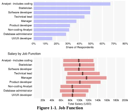
The 816 survey respondents mostly worked in data science or analytics
(80%), but also included some managers and other tech workers connected to the data space. Fifty-three countries were represented, with two-thirds of the respondents coming from across the U.S. About 40% of the respondents were from tech companies,1 with the rest coming from a wide range of industries
including finance, education, health care, government, and retail. Startup workers made up 20% of the sample, and 40% came from companies with over 2,500 employees. The sample was predominantly male (85%).
One of the more revealing results of the survey shows that respondents were less likely to self-identify as technical individual contributors than we expect from the general population of those working in data-oriented jobs. Only 41% were from individual contributors; 33% were tech leads or architects, 16% were managers, and 9% were executives. It should be noted, however, that the executives tended to be from smaller companies, and so their actual role might be more akin to that of the technical leads from the larger
companies (43% of executives were from companies with 100 employees or less, compared to 26% for non-executives). Judging by the tools used, which we’ll discuss later, almost all respondents had some technical role.
Figure 1-1. Job Function
We also asked participants about their benefits and working conditions; a majority were provided health care (94%) and allowed flex time (80%) and the option to telecommute (70%). The average work week of the sample was about 46 hours, with respondents in managerial and executive positions working longer weeks (49 and 52 hours, respectively). One-third of
Salary Report
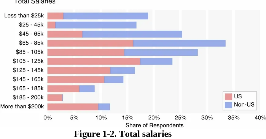
The median base salary of all respondents was $91k, rising to $98k for total salary (this includes the respondents’ estimates of their non-salary
compensation).2 For U.S. respondents only, the base and total medians were
$105k and $144k, respectively.
Figure 1-2. Total salaries
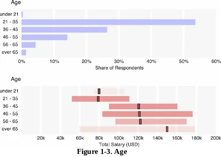
Certain demographic variables clearly correlate with salary, although since they also correlate with each other, the effects of certain variables can be conflated; for this reason, a more conclusive breakdown of salary, using regression, will be presented later. However, a few patterns can already be identified: in the salary graphs, the order of the bars is preserved from the graphs with overall counts; the bars represent the middle 50% of respondents of the given category, and the median is highlighted.3
Some discrepancies are to be expected: younger respondents (35 and under) make significantly less than the older respondents, and median salary
Figure 1-3. Age
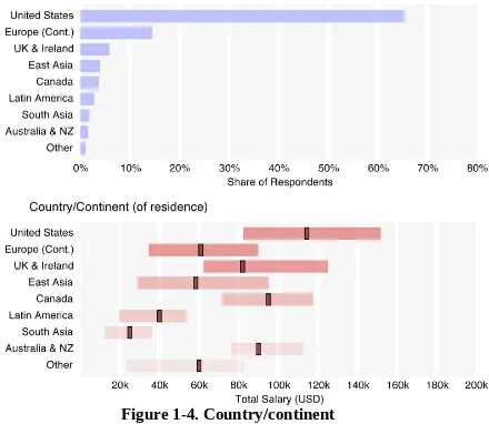
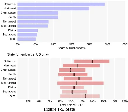
Median U.S. salaries were much higher than those of Europe ($63k) and Asia ($42k), although when broken out of the continent, the U.K. and Ireland rose to a median salary of $82k – more on par with Canada ($95k) and
Figure 1-5. State
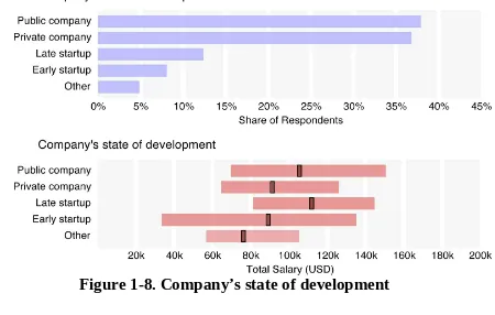
Major industries with the highest median salaries included banking/finance ($117k) and software ($116k). Surprisingly, respondents from the
Figure 1-8. Company’s state of development
Tool Analysis
Tool usage can indicate to what extent respondents embrace the latest developments in the data space. We find that use of newer, scalable tools often correlates with the highest salaries.
When looking at Hadoop and RDBMS usage and salary, we see a clear boost for the 30% of respondents who know Hadoop – a median salary of $118k for Hadoop users versus $88k for those who don’t know Hadoop. RDBMS tools do matter – those who use both Hadoop and RDBMSs have higher salaries ($122k) – but not in isolation, as respondents who only use RDBMSs and not Hadoop earn less ($93k).
Figure 1-9. Use of RDBMS and Hadoop
Tool Use in Data Today
While this general information about data tools can be useful, practitioners might find it more valuable to look at a more detailed picture of the tools being used in data today. The survey presented respondents with eight lists of tools from different categories and asked them to select the ones they “use and are most important to their workflow.” Tools were typically
programming languages, databases, Hadoop distributions, visualization applications, business intelligence (BI) programs, operating systems, or
statistical packages.4 One hundred and fourteen tools were present on the list,
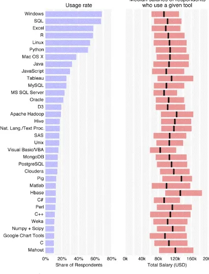
Figure 1-10. Most commonly used tools
data technology, there is no sign that SQL is going away.5 This year R and
Python were (just) trailing Excel, but these four make up the top data tools, each with over 50% of the sample using them. Java and JavaScript followed with 32% and 29% shares, respectively, while MySQL was the most popular database, closely followed by Microsoft SQL Server.
The most commonly used tool – whose users’ median salary surpassed $110k – was Tableau (used by 25% of the sample), which also stands out among the top tools for its high cost. The common usage of Tableau may relate to the high median salaries of its users; companies that cannot afford to pay high salaries are likely less willing to pay for software with a high per-seat cost. Further down the list we find tools corresponding to even higher median salaries, notably the open source Hadoop distributions and related
frameworks/platforms such as Apache Hadoop, Hive, Pig, Cassandra, and Cloudera. Respondents using these newer, highly scalable tools are often the ones with the higher salaries.
Figure 1-11. High-salary tools: median salaries of respondents who use a given tool
Also in line with last year’s data, the tools whose users tended to be from the lower end of the salary distribution were largely commercial tools such as SPSS and Oracle BI, and Microsoft products such as Excel, Windows,
one (or both) of these two tools was only $94k.
Figure 1-12. Low-salary tools: median salaries of respondents who use a given tool
Note that “tool median salaries” – that is, the median salaries of users of a given tool – tend to be higher than the median salary figures quoted above for demographics. This is not a mistake: respondents who reported using many
Tool Correlations
In addition to looking at how tools relate to salary, we also can look at how they correlate to each other, which will help us develop predictor variables for the regression model. Tool correlations help us identify established
ecosystems of tools: i.e., which tools are typically used in conjunction. There are many ways of defining clusters; we chose a strategy that is similar to that used last year6 but found more distinct clusters, largely due to the doubling of
the sample size.
The “Microsoft-Excel-SQL” cluster was more or less preserved (as “Cluster 1”), but the larger “Hadoop-Python-R” cluster was split into two parts. The larger of these, Cluster 2, is made up of Hadoop tools, Linux, and Java, while the other, Cluster 3, emphasizes coding analysis with tools such as R, Python, and Matlab. With a few tool omissions, it is possible to join Clusters 2 and 3 back into one, but the density of connections within each separately is
significantly greater than the density if they are joined, and the division allows for more tools to be included in the clusters. Cluster 4, centered
The only tool with over 35 users that did not fit into a cluster was Tableau: it correlated well with Clusters 1 and 2, which made it even more of an outlier in that these two clusters had the highest density of negative correlations (i.e., when variable a increases, variable b decreases) between them. In fact, all of the 53 significant negative correlations between two tools were between one tool from Cluster 1 and another from Cluster 2 (35 negative correlations), 3 (6), or 4 (12).
Most respondents did not cleanly correspond to one of these tool categories: only 7% of respondents used tools exclusively from one of these groups, and over half used at least one tool from four or five of the clusters. The meaning behind the clusters is that if a respondent uses one tool from a cluster, the chance that she uses another from that cluster increases. Many respondents
tended toward one or two of the clusters and used relatively few tools from the others.
Interpreting the clusters
source is perhaps the most important feature, dividing Cluster 1 from the others. Cluster 1 also contains Microsoft tools, although the producer of the tool does not necessarily determine cluster membership (MySQL and Oracle RDB are in different clusters).
The large number of tools in Cluster 2 is no anomaly: people working with Hadoop-like tools tend to use many of them. In fact, for tools such as EMR, Cassandra, Spark, and MapR, respondents who used each of these tools used an average of 18–19 tools in total. This is about double the average for users of some Cluster 1 tools (e.g., users of SPSS used an average of 9 tools, and users of Excel used an average of 10 tools). Some of the Cluster 2 tools complement each other to form a tool ecosystem: that is, these tools work best together, and might even require one another. From the perspective of individuals deciding which tools to learn next, the high salaries correlated with use of Cluster 2 tools is enticing, but it may be the case that not just one but several tools need to be learned to realize the benefits of such skills. Other tools in Cluster 2 are not complements to each other, but alternatives: for example, MapR, Cassandra, Cloudera, and Amazon EMR. The fact that even these tools correlate could be an indication of the newness of Hadoop: individuals and companies have not necessarily settled on their choice of tools and are trying different combinations among the many available options. The community nature of the open source tools in Cluster 2 may provide another explanation for why alternative tools are often used by the same respondents. That community element, plus the single-purpose nature of many of the open source tools, contrasts Cluster 2 with the more mature, and vertically integrated, proprietary tools in Cluster 1.
Some similar patterns exist in Clusters 1 and 3 as well, though perhaps not to the same extreme. For example, R and Python, while they are often used together, are capable of doing many of the same things (stated differently, many – even most – uses of either R or Python for data analysis can be done entirely by one). However, these two correlate very strongly with one
another. Similarly, business intelligence applications such as MicroStrategy, BusinessObjects, and Oracle BI correlate with each other, as do statistical packages SAS and SPSS. In what is a relatively rare cross-cluster bond between Clusters 1 and 3, R and SAS also correlate positively.7
versus BI analysts), it is also a sign that data workers often try different tools with the same function. Some might feel that the small set of tools they work with is sufficient, but they should know that this makes them outliers – and given the aforementioned correlation between number of tools used and
Regression Model of Total Salary
Continuing toward the goal of understanding how demographics, position, and tool use affect salary, we now turn to the regression model of total
salary.8 Earlier, we mentioned some one-variable comparisons, but there is an
important difference between those observations and this model: before there was no indication of whether a given discrepancy was attributable to the variable being compared or another one that correlates with it, but here observations about a variable’s effect on salary can be understood with the phrase “holding other variables constant.”
For each tool cluster, one variable was included in the potential predictors with a value equal to the number of this cluster’s tools used by a respondent. Demographic variables were given approximate ordinal values when
appropriate,9 and most variables that obviously overlapped with others were
omitted.10 From the 86 potential predictor variables, 27 were included in the
final model.11 The adjusted R-squared was .58: that is, approximately 58% of
the variation in salary is explained by the 27 coefficients.
Variable (unit) Coefficient in USD Industry: science and technology - – $17,294 Industry: government - – $16,616
Gender: female - – $13,167
Age per 1 year + $1,094
Years working in data per 1 year + $1,353
Doctorate degree - + $11,130
Company size per 1 employee + $0.90 Company age per 1 year, up to ~30 – $275 Company type: early startup - – $17,318 Cloud computing: no cloud use - – $12,994 Cloud computing: experimenting - – $9,196
Cluster 1 per 1 tool – $1,112
Cluster 2 per 1 tool + $1,645
Cluster 3 per 1 tool + $1,900
Bonus - + $17,457
Stock options - + $21,290
Stock ownership - + $14,709
Geography
Geography presented a few surprises: living (and, we assume, working) in Europe or Asia lowers the expected salary by $24k or $31k, respectively, while living in California, the Northeast, or the Mid-Atlantic states adds between $17k and $26k to the predicted salary. Working in education lowers the expected salary by a staggering $30k, while those in government and science and technology also have significantly lower salaries (by
Gender
Experience
Each year of age adds $1,100 to the expected salary, but each year of
experience working in data adds an additional $1,400. Thus, each year, even without other changes (e.g., in tool usage), the model will predict a data
analyst/engineer’s salary to increase by $2,500. This is slightly tempered by a subtraction of $275 for each year the respondent’s company has been in
business. This does not mean that brand-new startups have the best salaries, though: early startups (as opposed to late startups and private and public companies) impose a predictive penalty of $17k. Company size contributes a positive coefficient, adding an average of 90 cents per employee at the
Education and Position
Having a doctorate degree is a plus – it adds $11k, which is a similar bump to that experienced at each position level. From non-manager to tech lead, tech lead to manager, and manager to executive there is, on average, a $10k
increase. This might seem small, but it is coupled with another increase based on the percentage of time spent as a manager: each 1% spent as a manager adds $326. So, the difference in expected salary between a non-manager and an executive whose role is 100% managerial is about $63k (again, holding other variables constant – managers/executives tend to be older, further expanding this figure).
Hours Worked
Cloud Computing
Use of cloud computing provides a significant boost, with those not on the cloud at all earning $13k less than those that do use the cloud; for
respondents who were just experimenting with the cloud, the penalty was reduced by $4k. Here we should be especially careful to avoid assuming causality: the regression model is based on observational survey data, and we do not have any information about which variables are causing others. Cloud use very well may be a contributor to company success and thus to salary, or the skills needed to use tools that can run on the cloud may be in higher
demand, driving up salaries. A third alternative is simply that companies with smaller funds are less likely to use cloud services, and also less likely to pay high wages. The choice might not be one of using the cloud versus an in-house solution, but rather of whether to even attempt to work with the
volume of data that makes the cloud (or an expensive alternative) worthwhile.
Tool Use
Two of the clusters – 4 and 5 – were not sufficiently significant indicators of salary to be kept in the model. Cluster 1 contributed negatively to salary: for every tool used in this cluster, expected salary decreases by $1,112.
However, recall that respondents who use tools from Cluster 1 tend to use few tools, so this penalty is usually only in the range of $2k–$5k. It does mean, however, that respondents that gravitate to tools in Cluster 1 tend to earn less. (The median salary of respondents who use tools from Cluster 1 but not a single tool from the other four clusters is $82k, well below the overall median.)
Users of Cluster 2 and 3 tools fare better, with each tool from Cluster 2 contributing $1,645 to the expected total salary and each tool from Cluster 3 contributing $1,900. Given that tools from Cluster 2 tend to be used in greater numbers, the difference in Cluster 2 and 3 contributions is probably
negligible. What is more striking is that using tools from these clusters not only corresponds to a higher salary, but that incremental increases in the number of such tools used corresponds to incremental salary increases. This effect is impressive when the number of tools used from these clusters
Other Components
Finally, we can give approximations of the impact of other components of compensation. This is determined by a combination of how much (in the respondents’ estimation) each of these variables contributes to their salary, and any correlation effect between salary and the variable itself. For example, employees who receive bonuses might tend to earn higher salaries before the bonus: the compensation variables would include this effect. Earning bonuses meant, on average, a $17k increase in expected total salary, while stock
options added $21,290 and stock ownership added $14,709. Having no retirement plan was a $21,518 penalty.
The regression model presented here is an approximation, and was chosen not only for its explanatory power but also for its simplicity: other models we found had an adjusted R-squared in the .60–.70 range, but used many more variables and seemed less suitable for presentation. Given the vast amount of information not captured in the survey – employee performance, competence in using certain tools, communication or social skills, ability to negotiate – it is remarkable that well over half of the variance in the sample salaries was
Conclusion
This report highlights some trends in the data space that many who work in its core have been aware of for some time: Hadoop is on the rise; cloud-based data services are important; and those who know how to use the advanced, recently developed tools of Big Data typically earn high salaries. What might be new here is in the details: which tools specifically tend to be used together, and which correspond to the highest salaries (pay attention to Spark and
Storm!); which other factors most clearly affect data science salaries, and by how much. Clearly the bulk of the variation is determined by factors not at all specific to data, such as geographical location or position in the company hierarchy, but there is significant room for movement based on specific data skills.
As always, some care should be taken in understanding what the survey sample is (in particular, that it was self-selected), although it seems unlikely that the bias in this sample would completely negate the value of patterns found in the data as industry indicators. If there is bias, it is likely in the direction of the O’Reilly audience: this means that use of new tools and of open source tools is probably higher in the sample than in the population of all data scientists or engineers.
For future research we would like to drill down into more detail about the actual roles, tasks, and goals of data scientists, data engineers, and other people operating in the data space. After all, an individual’s contribution – and thus his salary – is not just a function of demographics, level/position, and tool use, but also of what he actually does at his organization.
The most important ingredient in continuing to pass on valuable information is participation: we hope that whatever you get out of this report, it is worth the time to fill out the survey. The data space is one that changes quickly, and we hope that this annual report will help the reader stay on its cutting edge.
1 The 40% tech company figure results from the combination of the industries
“software and application development,” “IT/systems/solutions
our audience choosing these categories typically come from (paradigmatic) tech companies. Some companies from other industries would also consider themselves tech companies (e.g., startups using advanced technology and operating in the entertainment industry).
2 Following standard practice, median figures are given (the right skew of the
salary distribution means that individuals with particularly high salaries will push up the average). However, since respondents were asked to report their salary to the nearest $10k, the median (and other quantile) calculations are based on a piecewise linear map that uses points at the centers and borders of the respondents’ salary values. This assumes that a salary in a $10k range has a uniform chance of having any particular value in that range. For this reason, medians and quantile values are often between answer choices (that is, even though there were only choices available to the nearest $10k, such as $90k and $100k, the median salary is given as $91k).
3 When the category subsample is small, the bar on the salary graph becomes
more transparent.
4 Two exceptions were “Natural Language/Text Processing” and
“Networks/Social Graph Processing,"” which are less tools than they are types of data analysis.
5 In comparing the Strata Salary Survey data from this year and last year, it is
important to note two changes. First, the sample was very different. The data from last year was collected from Strata conference attendees, while this year’s data was collected from the wider public. Second, in the previous survey only three tools from each category were permitted. The removal of this condition has dramatically boosted the tool usage rates and the number of tools a given respondent uses.
6 For cluster formation, only tools with over 35 users in the sample were
considered. Tools in each cluster positively correlated (at the α = .01 level using a chi-squared distribution) with at least one-third of the others, and no negative correlations were permitted between tools in a cluster. The one exception is SPSS, which clearly fits best into Cluster 1 (three of the five tools with which it correlates are in that group). SPSS was notable in that its users tended to use a very small number of tools.
7 Whether SAS and R are complements or rivals depends on who you ask.
been a recent push from SAS to allow for integration between these tools.
8 We had respondents earning more than $200k select a “greater than $200k”
choice, which is estimated as $250k in the regression calculation. This might have been advisable even had we had the exact salaries for the top earners (to mitigate the effects of extreme outliers). This does not affect the median statistics reported earlier.
9 For several of these ordinal variables, the resulting coefficient should be
understood to be very approximate. For example, data was collected for age at 10-year intervals, so a linear coefficient for this variable might appear to be predicting the relation between age and salary at a much finer level than it actually can.
10 Variables that repeat information, such as the total number of tools, are
typically omitted (there is too much overlap between this and the cluster tool count variables; the same goes for individual tool usage variables). One exception is position/role: the role percentages were kept in the pool of
potential predictor variables, including one variable describing the percentage of a respondent’s time spent as a manager (in fact, this was the only role variable to be kept in the final model). The respondent’s overall position (non-manager, tech lead, manager, executive) clearly correlates with the manager role percentage, but both variables were kept as they do seem to describe somewhat orthogonal features. While this may seeming confusing, this is partly due to the difference in the meaning of “manager” as a position or status, and “manager” as a task or role component (e.g., executives also “manage”).
11 Variables were included in or excluded from the model on the basis of
statistical significance. The final model was obtained through forward
stepwise linear regression, with an acceptance error of .05 and rejection error of .10. Alternative models found through various other methods were very similar (e.g., inclusion of one more industry variable) and not significantly superior in terms of predictive value.
12 The “level” units of position correspond to integers, from 0 to 4. Thus, to
1. Take the Data Science Salary and Tools Survey 2. Strata+Hadoop World
3. 1. 2014 Data Science Salary Survey a. Executive Summary