Laterally constrained inversion of helicopter-borne frequency-domain
electromagnetic data
Bernhard Siemon
a,⁎
, Esben Auken
b, Anders Vest Christiansen
ba
Federal Institute for Geosciences and Natural Resources, Stilleweg 2, 30655 Hannover, Germany
b
HydroGeophysics Group, Department of Earth Sciences, University of Aarhus, Høegh-Gulbergs Gade 2, 8000 Aarhus C, Denmark
Received 6 February 2007; accepted 13 November 2007
Abstract
Helicopter-borne frequency-domain electromagnetic (HEM) surveys are used for fast high-resolution, three-dimensional resistivity mapping. Standard interpretation tools are often based on layered earth inversion procedures which, in general, explain the HEM data sufficiently. As a HEM system is moved while measuring, noise on the data is a common problem. Generally, noisy data will be smoothed prior to inversion using appropriate low-pass filters and consequently information may be lost.
For the first time the laterally constrained inversion (LCI) technique has been applied to HEM data combined with the automatic generation of dynamic starting models. The latter is important because it takes the penetration depth of the electromagnetic fields, which can heavily vary in survey areas with different geological settings, into account. The LCI technique, which has been applied to diverse airborne and ground geophysical data sets, has proven to be able to improve the HEM inversion results of layered earth structures. Although single-site 1-D inversion is generally faster and—in case of strong lateral resistivity variations—more flexible, LCI produces resistivity—depth sections which are nearly
identical to those derived from noise-free data.
The LCI results are compared with standard single-site Marquardt–Levenberg inversion procedures on the basis of synthetic data as well as
field data. The model chosen for the generation of synthetic data represents a layered earth structure having an inhomogeneous top layer in order to study the influence of shallow resistivity variations on the resolution of deep horizontal conductors in one-dimensional inversion results. The field data example comprises a wide resistivity range in a sedimentary as well as hard-rock environment.
If a sufficient resistivity contrast between air and subsurface exists, the LCI technique is also very useful in correcting for incorrect system altitude measurements by using the altitude as a constrained inversion parameter.
© 2008 Elsevier B.V. All rights reserved.
Keywords: Laterally constrained inversion; Marquardt–Levenberg inversion; Helicopter-borne electromagnetics; Starting models; Resistivity sections;
Centroid depth
1. Introduction
Helicopter-borne electromagnetic (HEM) surveying enables resistivity mapping of large areas with high lateral resolution in a relative short time (Fraser, 1978). Since the introduction of the centroid depth (Sengpiel, 1988) it has been common practise to present the results from multi-frequency HEM systems not only
as apparent resistivity maps but also as resistivity-depth images called Sengpiel sections (Huang and Fraser, 1996). Today, ver-tical resistivity sections (VRS) and thematic maps displaying resistivities at certain depths below surface or sea level are derived from layered earth inversion models, which have been routinely produced for more than a decade (Fluche and Sengpiel, 1997).
Due to the limited extent of the HEM footprint (e.g. Beamish, 2003), which is of the order of the centroid depth values, i.e. less than 200 m in general, one-dimensional inver-sion of HEM data is often sufficient to explain the data in areas Journal of Applied Geophysics 67 (2009) 259–268
www.elsevier.com/locate/jappgeo
⁎Corresponding author. Tel.: +49 511 643 3488; fax: +49 511 643 3663.
E-mail address:[email protected](B. Siemon).
URL:http://www.bgr.bund.de/(B. Siemon).
where the subsurface resistivity distribution varies relatively slowly in lateral direction. Even moderately dipping conductors can be modelled this way (Sengpiel and Siemon, 2000; Jordan and Siemon, 2002). In case of strong lateral resistivity varia-tions, however, 1-D inversion of HEM data often fails to explain the data sufficiently and typical 3-D effects occur in the resis-tivity sections (Sengpiel and Siemon, 1998). Under such con-ditions extensive 3-D modelling is necessary using forward (e.g. Avdeev et al., 1998) or inverse (e.g.Sasaki, 2001) solutions.
As a HEM system is moved with relatively high speed while measuring, it is not possible to stack data sufficiently. Further-more, system noise is a common problem. This system noise level has been reduced after a number of hardware improvements during recent years, but even modern digital devices may have noise levels which are of the order of the data values measured when flying high or above highly resistive subsurface. Generally, noisy data will be smoothed prior to inversion using appropriate low-pass filters and consequently resistivity information may be lost. Inversion of unfiltered data, however, often leads to resis-tivity models with unacceptable variation from site to site. This can be detrimental if the resistivity models serve directly as input for geologic or hydrologic numerical modelling (e.g.Bakker et al., 2006). An alternative to smoothing the data is smoothing the resulting model parameters by careful averaging or by lateral parameter correlation (Tølbøll and Christensen, 2006; Tøbøll, 2007), which also allows adding a priori information derived from ground geophysical data or drill holes.
In this paper we introduce the laterally constrained inversion (LCI) of HEM data. Diverse LCI techniques have success-fully been adapted to geophysical data (e.g.Auken et al., 2000 (pulled array DC data); Auken and Christiansen, 2004 (2-D geoelectrical data);Monteiro Santos, 2004(ground frequency-domain electromagnetic (EM) data); Auken et al., 2004 (airborne time-domain EM data); Auken et al., 2005 (1-D geoelectrical data);Wisén et al., 2005(geoelectrical and bore-hole data); Wisén and Christiansen, 2005 (geoelectrical and surface wave seismic data);Tartaras and Beamish, 2006 (fixed-wing frequency-domain EM data)). The LCI procedure used here is adapted to a one-dimensional inversion code developed at the HydroGeophysics Group (HGG) of the University of Aarhus, Denmark (Auken et al., 2002). As the single-site inversion code has also been recently adapted to HEM data, both the single-site and the LCI inversion results will be compared with established inversion procedures developed at the Federal Institute for Geosciences and Natural Resources (BGR). For more than a decade these Marquardt–Levenberg inversion (MLI) procedures have successfully been used for the interpretation of thousands of line-km of HEM data (e.g. Sengpiel and Siemon, 1997; Siemon et al., 2002; Kirsch et al., 2003; Siemon et al., 2004; Eberle and Siemon, 2006).
The automatic calculation of reasonable starting models required by the MLI procedure is essential to economically invert huge data sets being typical in airborne surveys. The starting models used in this study will be derived from apparent resistivity vs. centroid depth sounding curves, which account for the pene-tration depth of the electromagnetic fields (Sengpiel and Siemon, 2000).
2. Methods
2.1. Calculations of HEM secondary field values
Helicopter-borne frequency-domain electromagnetic sys-tems use a small number of transmitter coils (up to 6) to gen-erate oscillating primary magnetic fields at discrete frequencies, which induce eddy currents in the subsurface. The correspond-ing secondary magnetic fields are measured with receiver coils at a lateral distance of up to 8 m. They depend on system parameters like frequencyf, transmitter–receiver coil separation
r, system altitudeh, and the resistivity ρof the subsurface. As the secondary fields are very small with respect to the primary fields, the primary fields are generally bucked out and the relative secondary fields Z are measured in parts per million (ppm). The secondary magnetic field is a complex quantity having in-phase (R) and quadrature (Q) components.
Solving the induction equation with respect to a horizontal-coplanar coil system over a layered subsurface and omitting the direct magnetic field leads to (e.g.Ward and Hohmann, 1987):
Z¼ðRþiQÞ ¼r3
where R0 is a complex reflection coefficient containing the underground vertical resistivity distributionρ(z) withzpointing vertically downwards,α0= (λ ρ0are the permittivity, permeability, and resistivity of free space (air layer), respectively,J0is the Bessel function of first kind and zeroth order, andi= (−1)1/2is the imaginary unit. It is assumed that the subsurface permittivity and permeability are the same as in the air layer and the transmitter and the receiver dipoles are in the same height,h, above the surface of the ground.
At BGR Eq. (1) is evaluated using the fast Hankel transform (FHT) (Johanson and Sørenson, 1979) with 92 filter coeffi-cients and 10 points per decade. A faster procedure based on a Laplace transform (LT), which needs 12 filter coefficients only was introduced byFluche (1990). Applying the LT to Eq. (1) requires the substitution k= α0h which causes thatJ0≈1 as long asr/hb0.3 (Mundry, 1984), i.e. only the first term of the Bessel series (J0(x)≈1−x2/ 4 +x4/ 64−…) is necessary. The LT is applicable ifrbh, but for small values ofh more terms of the Bessel series have to be used. At HGG Eq. (1) is evaluated using the FHT with 10 points per decade using the fast digital filter byChristensen (1990). The number of used filter coefficients depends on the convergence of the convolu-tion to a staconvolu-tionary sum.
2.2. Apparent resistivity and centroid depth
both components of the secondary field for the apparent resistivity calculation. The output parameters of this pseudo-layer half-space inversion (Fraser, 1978) are the apparent resistivity ρa and the apparent distance Da. The apparent
distance, i.e. the distance of the sensor from the top of the conducting half-space, can be greater or smaller than the measured sensor altitude h. The difference of both, which is called the apparent depthda=Da−h, is positive in case of a resistive cover (including an air layer containing the trees); otherwise a conductive cover exists above a more resistive substratum. From the apparent resistivity and the apparent depth, the centroid depth (Sengpiel, 1988), which is a measure of the mean penetration of the induced currents in the subsurface, is derived asz⁎=d
a+pa/ 2 withpa= 503.3 (ρa/f)
1/2
(Siemon, 2001). Each set of half-space parameters is obtained individually at each of the HEM frequencies and at each of the sampling points of a flight line.
2.3. Marquardt–Levenberg layered half-space inversion
The model parameters of the 1-D inversion are the resistivitiesρand thicknessestof the model layers (the thick-ness of the underlying half-space is assumed to be infinite). Several procedures for HEM data inversion have been published (e.g.Qian et al., 1997; Fluche and Sengpiel, 1997; Beard and Nyquist, 1998; Ahl, 2003; Huang and Fraser, 2003) which are often adapted from algorithms developed for ground EM data. At BGR the Marquardt–Levenberg inversion proce-dure is used, which searches for the smoothest model fitting the data (Sengpiel and Siemon, 1998, 2000). The integral contain-ing the Bessel function is solved by applycontain-ing the FHT or LT and singular value decomposition (SVD) is used to invert the matrices (Fluche and Sengpiel, 1997). The MLI inversion pro-cedure is stopped when a given relative change threshold is reached. This threshold is defined as the differential fit of the modelled data to the measured HEM data. Noise is not taken into account and we normally use a 10% threshold for field data and a 1% threshold for synthetic data, i.e. the inversion stops when the enhancement of the relative fit for each of the last three iteration steps is less than 10% or 1%, respectively.
2.4. Laterally constrained layered half-space inversion
The laterally constrained inversion scheme is described in detail in Auken and Christiansen (2004) and in Auken et al. (2005)and therefore the following is a conceptual summary.
The LCI model is a section of stitched-together 1-D models along the profile. The lateral distances between the models are determined by the sampling density of the data and may be non-equidistant. The primary model parameters are layer resistivities and thicknesses but the lateral constraints might as well be applied on the depths. The forward modelling is done by cal-culating the vertical secondary magnetic field from a vertical magnetic dipole over a layered half-space following Eq. (1).
The inversion procedure is stopped when the decrease in total residual is less than 0.5% from one iteration to the next. To make the inversion robust to the starting model the inversion is guided in the sense that the maximum change of any parameter
is limited at each iteration. The step length is increased if an update of the model leads to a decreased residual but if an update leads to an increased residual the step length is decreased by increasing the damping. This damping scheme is robust to the starting model but at the expense of the number of iterations. The flight altitude for airborne data may be included as an inversion parameter with an a priori value determined from e.g. laser altimeters mounted on the sensor. Furthermore, the alti-tudes at neighbouring models are constrained laterally claming that they have to be equal within some limits. Including the flight altitude as an inversion parameter is beneficial as erro-neous measured altitudes will strongly influence the determina-tion of the near-subsurface resistivity structures.
All data sets are inverted simultaneously, minimizing a common objective function including the lateral constraints. Consequently, the output models are formed from a balance between the constraints, the physics of the method and the actual data. Model parameters with little influence on the data will be controlled by the constraints and vice versa. Due to the lateral constraints, information from one model will spread to neighbouring models.
The laterally constrained inversion is an over-determined problem. Therefore, we can calculate a sensitivity analysis of the model parameters, which is essential to assess the resolution of the inverted model (Tarantola and Valette, 1982).
2.5. Starting models
Due to the huge number of inversion models to be calculated in an airborne survey, it is beneficial to generate good starting models not too far from the true model as it stabilises the inversion and the inversion procedure requires less iterations to converge to the global minimum of the objective function. The capability to find the true model depends on the regularisation scheme and the model type.
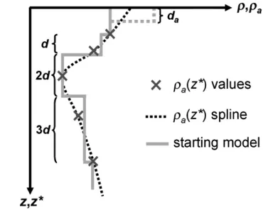
In order to construct starting models close to the true models, the starting models are derived from apparent resistivity vs. centroid depth sounding curves represented by polynomials or (smoothing) splines through theρa(z⁎) values (Fig. 1). The first (upper) and last (lower) layer boundaries are given by the
Fig. 1. Construction of starting models: the starting model is derived fromρa(z⁎)
sounding curves represented by a spline function through theρa(z⁎) values with
centroid depth values of the highest and lowest frequency, respectively. The intermediate layer boundaries result from linearly increasing layer thicknesses, where the thickness of the second layer is used as an increment for the following layers, i.e. the thickness of the third layer is twice the thickness of the second layer, the thickness of the fourth layer is three times the thickness of the second layer, etc. The corresponding resistivity values are taken from the apparent resistivity values of the highest and lowest frequency for the upper and lower layer, respectively, and the others are picked from ρa(z⁎) sounding curve at depths representing the layer centres. These starting models may be shifted up- or downwards and compressed or stretched by choosing factors less or greater than 1.0 for the upper or lower boundaries.
Optionally, a highly resistive top layer may be added. The resistivity of this top layer is set to e.g. 10 000 Ωm and the thickness is derived from the apparent depth da of the highest frequency used for the inversion as long as it is greater than a minimum depth value (e.g. 1 m). Otherwise the minimum depth value is used. The introduction of a resistive top layer is useful if a rather thin, i.e. less than the centroid depth of the highest frequency, resistive cover exists, e.g. dry sand above the water table or an air layer due to the canopy effect (Beamish, 2002). In that case, information about the existence of a resistive cover is provided by
da, but not byρa.
3. Results
The LCI results are compared with standard single-site inversion procedures on the basis of synthetic data as well as field data. The model chosen for the generation of synthetic data represents a layered earth structure having an inhomogeneous top layer in order to study the influence of shallow resistivity variations on the appearance of deep horizontal conductors in one-dimensional inversion results. The field data example comprises a wide resis-tivity range in a sedimentary as well as hard-rock environment.
3.1. Inversion of synthetic data
3.1.1. Forward calculations
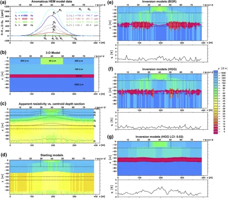
The synthetic data set used for the comparison was derived from a 3-D resistivity model consisting of a four-layer model with layer resistivities of 200, 100, 5, and 1000Ωm and thicknesses of 20, 30, and 10 m. The top contains a cube of 100 m × 500 m × 20 m of 50Ωm at 0–20 m depth (cf.Fig. 2b). The cell sizes of the 3-D model are 10 m along profile, 20 m across profile and 2 m in vertical direction. The third layer and the cube are denoted as deep and shallow conductor, respectively. The HEM data were calcu-lated with a step width of 5 m using X3Da (Avdeev et al., 1998) for a five-frequency (387, 1820, 8225, 41,550, and 133,200 Hz) horizontal-coplanar HEM system at a sensor altitude ofh= 30 m and a coil separation ofr= 8 m.
Exact inversion results are obtainable only if the forward modelling codes used by the inversion procedures are identical to those used for calculating the input synthetic data. As the synthetic data were derived by a numerical 3-D modelling code, small discrepancies between forward and inverse modelling are
normal, particularly if the resistivities vary laterally.Tables 1 and 2 list the HEM values obtained by the 3-D modelling (X3Da) above the normal structure and the centre of the model, respectively, in comparison with 1-D results to be expected there using procedures based on FHT and LT. These 3-D numerical values differ slightly from the 1-D values calculated with the different modelling codes, maybe due to different procedures for evaluating the integral describing the secondary field or by different rounding accuracies used. Above the centre of the model, differences between 3-D and 1-D modelling (Table 2) are obvious due to limited extent of the cube in profile direction (100 m).
The anomalous secondary field values with 1–5 ppm random noise added to the HEM data of the lowest to highest frequency, respectively, are displayed inFig. 2a. The normal field values, i.e. the secondary fields belonging to the layered half-space at sufficient distance from the shallow conductor, are shown in the legend and inTable 1.
3.1.2. Inversion of noisy data
The apparent resistivity vs. centroid depth cross-section (Fig. 2c), where 79 columns of colour-coded ρa(z⁎) sounding curves are stitched together, roughly reveals the conductors directly below the surface (shallow conductor) and below 50 m depth (deep conductor). The latter appears too thick and too resistive, and seems to be interrupted below the shallow conductor, where a more resistive, upwards tending zone occurs at depth.
The four-layer starting models (Fig. 2d) show the deep conductor also too thick and too resistive, although the resistivity of the third layer representing the deep conductor appears to be slightly decreased compared to theρa(z⁎) section around 60 m depth. This is due to overshooting of the spline function used for the construction of the starting models, which is not as smooth as the spline function used for the calculation of theρa(z⁎) sounding curves ofFig. 2c.
Four-layer inversion models are shown in Fig. 2e–g. The model sections consist of 79 columns of colour-coded 1-D models being stitched together. The relative misfit q of the inversion displayed below the model sections is defined by:
q½ ¼k 100
wherediand miare the complex input (measured or synthetic HEM data) and output (inverted model parameters), respec-tively, belonging to theNfrequencies used.
three-dimensionality of the model data. A further reduction of the threshold leads to more extreme models where the deep conductor becomes thinner and the resistivity of the fourth layer (half-space) often increases to values far above 1000Ωm. Using the HGG 1-D inversion code without any constraints and relative standard deviations between 0.01 and 0.05 for the
lowest and highest frequency data, respectively, leads to similar results, but the thickness of the third layer is less varying and the misfitqis a little bit smaller, particularly for those models close to the shallow conductor (Fig. 2f). Choosing smaller relative standard deviations results in thicker bulges outside and thinner layer thicknesses of the deep conductor inside the area of the
Table 1
HEM data derived by diverse 1-D forward modelling procedures (BGR: FHT (Fast Hankel Transform) and LT (Laplace Transform), HGG: FHT) for a four-layer half-space with resistivities of 200, 100, 5, and 1000Ωm and thicknesses of 20, 30, and 10 m; sensor altitudeh= 30 m; coil separationr= 8 m
BGR (FHT) BGR (LT) HGG (FHT) X3Da
f[Hz] R[ppm] Q[ppm] R[ppm] Q[ppm] R[ppm] Q[ppm] R[ppm] Q[ppm]
387 21.80 68.36 21.77 68.62 21.80 68.44 22.10 68.75
1820 129.1 164.4 129.1 164.4 129.2 164.7 129.8 164.6
8225 280.4 291.5 280.4 291.5 280.8 292.4 281.6 291.7
41,550 734.7 747.4 734.8 747.6 736.4 750.8 735.2 747.7
133,200 1506 1047 1509 1052 1512 1053 1515 1047
The numerical 3-D modelling results (X3Da) are obtained 150 m laterally apart from the boundary of the shallow conductor.
Fig. 2. Inversion of synthetic HEM data: a) Anomalous HEM data (1–5 ppm random noise added to HEM data of lowest–highest frequency), sensor altitudeh= 30 m
and coil separation r= 8 m; b) Four-layer half-space with resistivities of 200, 100, 5, and 1000 Ωm and thicknesses of 20, 30, and 10 m, containing a 100 m × 500 m × 20 m cube of 50Ωm at 0–20 m depth; c) Apparent resistivity vs. centroid depth cross-section (dots = centroid depth values); d) Four-layer starting
models derived fromρa(z⁎); e) MLI (LT) results (BGR); f ) MLI (FHT) results (HGG); g) LCI results (HGG). In addition, the boundaries of the original model (dashed
shallow conductor, i.e. the final models converge to the BGR MLI case. Again, the thickness of the shallow conductor appears to be 20–25% too small.
The laterally constrained inversion with horizontal con-straints of a factor of 1.02 for all model parameters results in smooth models which are quite homogeneous for the lower two layers which resemble the true model quite well (Fig. 2g). The side effects caused by the 3-D shallow conductor occurring particularly in the second layer are a bit smoother than in the MLI sections. The thickness of the shallow conductor appears to be about 25% too small, even at the centre of the cube. Although the misfit is higher, the improvement of LCI compared with single-site inversions is obvious.
3.1.3. Handling of large data sets
As LCI computation time increases dramatically when the number of model parameters exceeds about 1000 (Table 3), large HEM data sets have to be divided into subsets. The increase in computation time is due to the current implementa-tion of the LCI algorithm which does not store the Jacobian matrix sparse but uses a straight forward Cholesky decomposi-tion to invert the matrix as discussed inChristiansen and Auken (2004). The HEM subsets are inverted individually and lateral discrepancies in resistivity and depth may occur at the boundaries of the subsets. This effect is studied now on synthetic data.
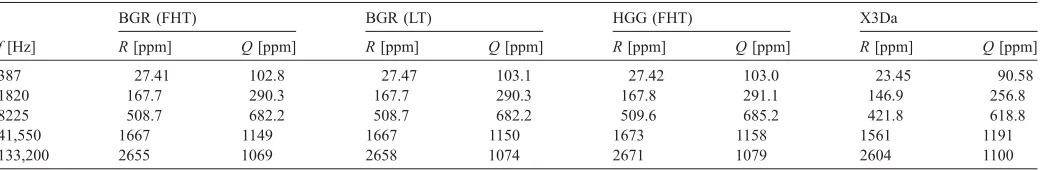
InFig. 2g, LCI simultaneously took all the 79 models into account. Subsets of only 20 models (19 for the last subset) were used to achieve the results shown in Fig. 3a. The results are similar but blocky.
Using an overlap of e.g. 50%, i.e. the last and first ten models of each neighbouring twenty-model subsets were weighted averaged with respect to their distance from the centre of the subsets, resulted in a bit smoother model suite (Fig. 3b) compared with that of Fig. 3a. The minimum overlap is a compromise between computation time and footprint; it normally should be of the order of 100 m, i.e. a point separation of 4–5 m requires an overlap O of 20–25 models for each subset. The number of subsetsS to be calculated consisting of
M models increases from S to (SM− O) / (M − O), i.e. the computation time nearly doubles for a 50% overlap and a large number of subsets.
Next, we added a priori information from the last model in the previous section to the first model in the next section causing that the two models close to a subset boundary are forced to be very similar. This does not marginally change the computation time. The disadvantage, however, is that the constraints at the boundaries are directional, i.e. we got different results when progressing in different directions along a profile. Therefore, the constraints have to be meticulously chosen and checked by inverting in both directions and that will double the computation time.
Finally, we applied a priori constraints on both sides, i.e. to the first and last model, of each of the LCI subsets. The a priori constraints had to be derived beforehand by LCI of individual subsets (denoted as a priori subsets) around the boundaries of the actual LCI subsets. The number of models necessary for the a priori subsets depends on the variations in the HEM data. The length of a profile section representing the a priori subsets should be in the order of the footprint. InFig. 3c, we used 40 Table 2
HEM data derived by diverse 1-D procedures (cf.Table 1) for a four-layer half-space with resistivities of 50, 100, 5, and 1000Ωm and thicknesses of 20, 30, and 10 m; sensor altitudeh= 30 m; coil separationr= 8 m
BGR (FHT) BGR (LT) HGG (FHT) X3Da
f[Hz] R[ppm] Q[ppm] R[ppm] Q[ppm] R[ppm] Q[ppm] R[ppm] Q[ppm]
387 27.41 102.8 27.47 103.1 27.42 103.0 23.45 90.58
1820 167.7 290.3 167.7 290.3 167.8 291.1 146.9 256.8
8225 508.7 682.2 508.7 682.2 509.6 685.2 421.8 618.8
41,550 1667 1149 1667 1150 1673 1158 1561 1191
133,200 2655 1069 2658 1074 2671 1079 2604 1100
The numerical 3-D modelling results are obtained above the centre of the shallow conductor.
Table 3
Comparison of computation times on a 2.8 GHz Pentium 4 PC for the inversion of five-frequency HEM field data (cf.Fig. 4, n.s. = not shown); LCI with 0.1–0.5
relative standard deviation (STD) and constrains of factor of 1.1 for the lower three layers
Figure Algorithm Remarks Number of layers Parameters per inversion Number of inversions Computation time [s]
4d BGR MLI (LT) 10% threshold 4 9 1500 26
n. s. BGR MLI (FHT) 10% threshold 4 9 1500 257
4e HGG MLI (FHT) 0.1–0.5 STD 4 9 1500 210
n. s. HGG LCI (FHT) 20 (AP= 20) models 4 180/180 75 + 74 167
4f HGG LCI (FHT) 50 (AP= 26) models 4 450/208 30 + 29 254
n. s. HGG LCI (FHT) 100 (AP= 26) models 4 900/208 15 + 14 760
n. s. HGG LCI (FHT) 200 (AP= 26) models 4 1800/208 8 + 7 3000
4g HGG LCI (FHT) 50 (AP= 26) models 3 +h 400/208 30 + 29 96
models, i.e. 200 m profile sections, for the a priori subsets and 20 models for the regular LCI subsets. The results are comparable to those of Fig. 2g, but the computing time increased from 26 to 39 s.
3.2. Inversion of field data
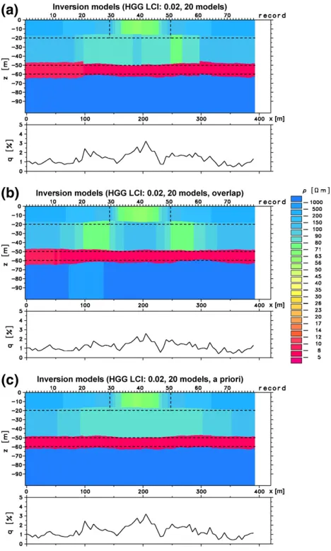
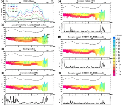
The example field data set used for comparing the inversion techniques is taken from a BGR survey in northern Sumatra in 2005 (Siemon et al., 2007). The HEM data was recorded with a five-frequency digital device (f= 387 Hz−133 kHz,r≈7.92 m) along a profile across a fresh-water lens. The profile section is 6.5 km long and contains 1500 records (= 15 fiducials) resulting in a sampling distance of 4.3 m on average. Based on calibration factors provided by the manufacturer (Fugro Airborne Surveys) and correction factors obtained over sea water the HEM system was carefully calibrated and recent HEM levelling techniques (Siemon, 2009-this issue) were applied to remove system drifts due to thermal variations. The data values shown inFig. 4a have
not been smoothed by low-pass filtering, i.e. they are noisy, but the noise is very small (the standard deviations are of the order of 1–3 ppm,Table 4).
The apparent resistivity vs. centroid depth section (Fig. 4b) reveals a fresh-water lens (ρa ≈25 Ωm) above saline water (ρa≈3Ωm) in alluvial sandy to clayey sediments. To the north-west where fish ponds exist close to the shoreline apparent resistivities drop below 1 Ωm indicating the occurrence of saltwater, and to the south-east moderate to high apparent resistivities indicate volcanic hard rocks containing fresh water (Siemon et al., 2007).
The starting models consist of four layers with a highly resistive layer on top (Fig. 4c). The highly resistive top layer is introduced in order to compensate for an incorrect altitude determination caused by obstacles like buildings and trees. The calculated ground elevation–the topographic relief–may also be elevated, because it is derived from the difference of the system elevation (GPS-Z) and system altitude (laser altimeter). The inversion results obtained from the HEM data of Fig. 4a using single-site MLI are shown inFig. 4d (BGR LT) and Fig. 4e (HGG FHT). The single-site inversion results are very similar but not identical due to individual inversion designs like threshold values for the termination of the itera-tion process, regularisaitera-tion parameters, standard deviaitera-tion of the field data, etc. The threshold value for the BGR MLI using the LT was set to 10%. In order to get comparable inversion results the relative standard deviation on the field data values used by the HGG code was set to 0.1 times the frequency number, i.e. 0.1 for the lowest and 0.5 for the highest frequency. Increasing these values results in inversion models which are closer to the starting models and, on the other hand, smaller threshold values can cause extreme and sometimes oscillating inversion models. Both sections show slightly noisy resistivity models having thin to broad vertical stripes within the section.
The LCI results of Fig. 4f demonstrate that a smooth resistivity-depth section can be obtained even from noisy field data. The LCI approach uses sets of 50 data points and a priori constraints based on 26 data points. The lateral constraints were set to a factor of 1.1 except for the upper layer. Here the parameters are unconstrained to account for highly variable thicknesses and resistivities to be expected in the top layer due to obstacles above the surface of the earth. The thickness of this resistive top layer, however, affects the elevations of the layer boundaries below, because the depths below surface are laterally constrained and not the elevations.
Therefore, three-layer LCI results (Fig. 4g) were derived from starting models without a highly resistive top layer. Instead, the laser altitude is incorporated in the inversion as a model parameter. This approach saves one model parameter (altitude instead of resistivity and thickness of the top layer) to be calculated and provides reasonable altitude data. This effect can be observed where the highly resistive top layer (dark blue coloured inFig. 4f) vanishes inFig. 4g providing a smooth topographic relief.
The LCI computation time is of the order of those of the single-site inversions using FHT, but LCI is definitely slower compared to the single-site inversions using LT (Table 3). If the Fig. 3. Laterally constrained inversion results derived from noisy data: a)
number of models per subset is small, e.g. 20 models, the inversion result will still be noisy. Taking a sampling distance of about 4.3 m into account, a 20-model section is about 86 m long and that is, in general, smaller than the footprint. For large model subsets, however, the LCI computation time strongly increases with the number of models used in the subsets. Thus,
choosing 50 models per subset with 25 models overlap or a priori constraints based on 26 data points is a compromise between computation time and smoothing. A subset of 26 models corresponds to a profile section of about 112 m, and that is of the order of the footprint.
4. Discussion and conclusions
For the first time the laterally constrained inversion tech-nique has been applied to helicopter-borne frequency-domain electromagnetic data. It successfully combines the LCI tech-nique used for the interpretation of diverse airborne and ground geophysical data sets with the automatic generation of dynamic starting models. The latter is important because it takes the penetration depth of the EM fields, which can heavily vary in survey areas with different geological settings, into account. Table 4
Standard deviationsΔRandΔQof the field data shown inFig. 4after high-pass filtering (filter length: 40 values≈170 m)
f[Hz] ΔR[ppm] ΔQ[ppm]
387 1.2 1.2
1820 1.4 1.0
8232 2.1 1.7
41,550 2.2 1.4
133,200 3.2 2.5
Fig. 4. Field example: a) Five-frequency HEM data obtained along a NW–SE profile in Northern Sumatra in 2005; b) Apparent resistivity vs. centroid depth cross-section; c)
The laterally constrained inversion of both synthetic data and field data definitely improves the one-dimensional inversion results of layered earth structures. Even in case of noisy data LCI produces smooth resistivity-depth sections which are nearly identical to those derived from noise-free data. Thus, HEM data values need not be smoothed prior to inversion using LCI.
Non-layered earth structures, however, may be smoothed too much by LCI. If the inhomogeneities appear in a small number of layers only, e.g. in the top layer, where the constraints are chosen to be very weak, LCI may still provide improved in-version results. Currently, LCI is designed to apply lateral constraints on layer resistivities and depths. That may cause artefacts like undulating, surface-parallel layers. Further im-provements may be achieved applying constraints on elevations instead of depths in order to encourage horizontal structures below an undulating topographic relief.
Single-site 1-D inversion, on the other hand, is faster than LCI, particularly if the LT is used (Table 3). Single-site inver-sion is also more flexible in case of lateral resistivity variations, but the inversion results are often very noisy. It therefore de-pends on what the inversion results will be used for and in which step of the data processing we are. In the field one like to produce fast results using LT whereas in the office the computer power is larger and the speed is not decisive. If the HEM inversion models are directly used as input for e.g. 3-D hydrau-lic simulations, smoothing is always beneficial.
Measuring accurate system altitudes is a problem in airborne surveys, because the system, which is also a platform for the (laser) altimeter, may dip or tilt yielding increased altitudes or the canopy effect may cause decreased altitude values. Correction procedures are very useful for reducing major alti-tude errors, but minor ones may still be on the data used for inversion. The inversion procedures discussed in this paper compensate for an incorrect altitude determination by introdu-cing a resistive (air) top layer (BGR codes) or using the altitude as an inversion parameter (HGG codes). The first technique will only be able to provide reasonable results if the altitude mea-sured is smaller than its correct value; otherwise it requires correction for system attitude. The latter technique is faster, because only one additional parameter has to be calculated, and particularly if the altitude values are laterally constrained, it will provide reasonable results in cases of strong resistivity contrasts between air and subsurface. On the other hand, it will fail if the shallow subsurface is highly resistive or the topographic relief is very rough. If depths are laterally constrained, the altitude has to be an inversion parameter. Otherwise the elevations of the layer boundaries will be shifted downward in case of a resistive top layer (air). Therefore, it depends on the subsurface resistivity distribution, the altitude corrections facilities available, the topo-graphic relief, and the inversion procedure used which technique should be favoured.
Acknowledgements
We would like to thank the guest editor N. B. Christensen and an unknown reviewer as well as our Danish and German colleagues for thoroughly reviewing the manuscript.
References
Ahl, A., 2003. Automatic 1D inversion of multifrequency airborne electro-magnetic data with artificial neural networks: discussion and case study. Geophysical Prospecting 51, 89–97.
Auken, E., Christiansen, A.V., 2004. Layered and laterally constrained 2D inversion of resistivity data. Geophysics 69, 752–761.
Auken, E., Sørensen, K., Thomsen, P., 2000. Lateral constrained inversion (LCI) of profile oriented data—the resistivity case. Proceedings of the EEGS-ES,
Bochum, Germany, EL06.
Auken, E., Nebel, L., Sørensen, K., Breiner, M., Pellerin, L., Christensen, N.B., 2002. EMMA—a geophysical training and education tool for electromagnetic
modeling and analysis. Journal of Environmental & Engineering Geophysics 7, 57–68.
Auken, E., Christiansen, A.V., Jacobsen, L., Sørensen, K.I., 2004. Laterally constrained 1D-inversion of 3D TEM data. Extended Abstracts Book, 10th meeting EEGS-NS, Utrecht, The Netherlands.
Auken, E., Christiansen, A.V., Jacobsen, B.H., Foged, N., 2005. Piecewise 1-D laterally constrained inversion of resistivity data. Geophysical Prospecting 53, 497–506.
Avdeev, D.B., Kuvshinov, A.V., Pankratov, O.V., Newman, G.A., 1998. Three-dimensional frequency-domain modelling of airborne electromagnetic responses. Exploration Geophysics 29, 111–119.
Bakker, M., Bosch, A., Gunnink, J., 2006. Groningen valley. BurVal Working Group: Groundwater Resources in Buried Valleys—A Challenge for Geosciences.
Leibniz Institute for Applied Geosciences, Hannover, pp. 241–250.
Beamish, D., 2002. The canopy effect in airborne EM. Geophysics 67, 1720–1728.
Beamish, D., 2003. Airborne EM footprints. Geophysical Prospecting 51, 49–60.
Beard, L.P., 2000. Comparison of methods for estimating earth resistivity from airborne electromagnetic measurements. Journal of Applied Geophysics 45, 239–259.
Beard, L.P., Nyquist, J.E., 1998. Simultaneous inversion of airborne electromagnetic data for resistivity and magnetic permeability. Geophysics 63, 1556–1564.
Christensen, N.B., 1990. Optimized fast Hankel transform filters. Geophysical Prospecting 38, 545–568.
Christiansen, A.V., Auken, E., 2004. Optimizing a layered and laterally constrained 2D inversion of resistivity data using Broyden's update and 1D derivatives. Journal of Applied Geophysics 56, 247–261.
Eberle, D.G., Siemon, B., 2006. Identification of buried valleys using the BGR helicopter-borne geophysical system. Near Surface Geophysics 4, 125–133.
Fluche, B., 1990. Verbesserte Verfahren zur Lösung des direkten und inversen Problems in der Hubschrauber-Elektromagnetik. In: Haak, V., Hormilius, J. (Eds.), Protokoll Kolloquium Erdmagnetische Tiefensondierung, Hornburg, pp. 249–266.
Fluche, B., Sengpiel, K.-P., 1997. Grundlagen und Anwendungen der Hubschrauber-Geophysik. In: Beblo, M. (Ed.), Umweltgeophysik, Ernst und Sohn, Berlin, pp. 363–393.
Fraser, D.C., 1978. Resistivity mapping with an airborne multicoil electro-magnetic system. Geophysics 43, 144–172.
Huang, H., Fraser, D.C., 1996. The differential parameter method for multifrequency airborne resistivity mapping. Geophysics 61, 100–109.
Huang, H., Fraser, D.C., 2003. Inversion of helicopter electromagnetic data to a magnetic conductive layered earth. Geophysics 68, 1211–1223.
Johanson, H.K., Sørenson, K., 1979. Fast Hankel transforms. Geophysical Prospecting 27, 876–901.
Jordan, H., Siemon, B., 2002. Die Tektonik des nordwestlichen Harzrandes-Ergebnisse der Hubschrauber-Elektromagnetik. Zeitschrift der deutschen geologischen Gesellschaft 153, 31–50.
Kirsch, R., Sengpiel, K.-P., Voss, W., 2003. The use of electrical conductivity mapping in the definition of an aquifer vulnerability index. Near Surface Geophysics 1, 13–19.
Monteiro Santos, F.A., 2004. 1-D laterally constrained inversion of EM34 profiling data. Journal of Applied Geophysics 56, 123–134.
Mundry, E., 1984. On the interpretation of airborne electromagnetic data for the two-layer case. Geophysical Prospecting 32, 336–346.
Geophysics Workshop, Laboratory of Advanced Subsurface Imaging (LASI), Univ of Arizona, Tucson, CD-ROM.
Sasaki, Y., 2001. Full 3D inversion of electromagnetic data on PC. Journal of Applied Geophysics 46, 45–54.
Sengpiel, K.-P., 1988. Approximate inversion of airborne EM-data from a multilayered ground. Geophysical Prospecting 36, 446–459.
Sengpiel, K.-P., Siemon, B., 1997. Hubschrauberelektromagnetik zur Grundwasser-erkundung in der Namib-Wüste. Zeitschrift für angewandte Geologie 43, 130–136.
Sengpiel, K.-P., Siemon, B., 1998. Examples of 1D inversion of multifrequency AEM data from 3D resistivity distributions. Exploration Geophysics 29, 133–141.
Sengpiel, K.-P., Siemon, B., 2000. Advanced inversion methods for airborne electromagnetic exploration. Geophysics 65, 1983–1992.
Siemon, B., 2001. Improved and new resistivity-depth profiles for helicopter electromagnetic data. Journal of Applied Geophysics 46, 65–76.
Siemon, B., 2009. Levelling of helicopter-borne frequency-domain electro-magnetic data. Journal of Applied Geophysics 67, 209–221 (this issue).
doi:10.1016/j.jappgeo.2007.11.001.
Siemon, B., Stuntebeck, C., Sengpiel, K.-P., Röttger, B., Rehli, H.-J., Eberle, D.G., 2002. Investigation of hazardous waste sites and their environment using the BGR helicopter-borne geophysical system. Journal of Environ-mental & Engineering Geophysics 7, 169–181.
Siemon, B., Eberle, D.G., Binot, F., 2004. Helicopter-borne electromagnetic investigation of coastal aquifers in North-West Germany. Zeitschrift für Geologische Wissenschaften 32, 385–395.
Siemon, B., Steuer, A., Meyer, U., Rehli, H.-J., 2007. HELP ACEH–A
post-tsunami helicopter-borne groundwater project along the coasts of Aceh, northern Sumatra. Near Surface Geophysics 5, 231–240.
Tarantola, A., Valette, B., 1982. Generalized nonlinear inverse problem solved using the least squares criterion. Reviews of Geophysics and Space Physics 20, 219–232.
Tartaras, E., Beamish, D., 2006. Laterally constrained inversion of fixed-wing frequency-domain AEM data. Proceedings of Near Surface 2006, Helsinki, B019.
Tøbøll, R.J., 2007. The application of frequency-domain helicopter-borne electromagnetic methods to hydrogeological investigations in Denmark. PhD thesis. Department of Earth Sciences, University of Aarhus, Denmark. Tølbøll, R.J., Christensen, N.B., 2006. Robust 1D inversion and analysis of
helicopter electromagnetic (HEM) data. Geophysics 71, G53–G62.
Ward, S.H., Hohmann, G.W., 1987. Electromagnetic theory for geophysical applications. In: Nabighian, M.N. (Ed.), Electromagnetic Methods in Applied Geophysics —Theory, Volume 1, Investigations in Geophysics
No. 3. Society of Exploration Geophysicists, Tulsa, pp. 131–311.
Wisén, R., Christiansen, A.V., 2005. Laterally and mutually constrained inversion of surface wave seismic data and resistivity data. Journal of Environmental & Engineering Geophysics 10, 251–262.