SPATIAL AND TEMPORAL ANALYSIS OF SEA SURFACE SALINITY USING
SATELLITE IMAGERY IN GULF OF MEXICO
S. Rajabi a , M. Hasanlou a,*, A. R. Safari a
a School of Surveying and Geospatial Engineering, College of Engineering, University of Tehran, Tehran, Iran (saeed_rajabi, hasanlou, asafari)@ut.ac.ir
KEY WORDS: Sea surface salinity, Aquarius, Sea surface temperature, Chlorophyll-a concentration, Gulf of Mexico, Monitoring
ABSTRACT:
The recent development of satellite sea surface salinity (SSS) observations has enabled us to analyse SSS variations with high spatiotemporal resolution. In this regards, The Level3-version4 data observed by Aquarius are used to examine the variability of SSS in Gulf of Mexico for the 2012-2014 time periods. The highest SSS value occurred in April 2013 with the value of 36.72 psu while the lowest value (35.91 psu) was observed in July 2014. Based on the monthly distribution maps which will be demonstrated in the literature, it was observed that east part of the region has lower salinity values than the west part for all months mainly because of the currents which originate from low saline waters of the Caribbean Sea and furthermore the eastward currents like loop current. Also the minimum amounts of salinity occur in coastal waters where the river runoffs make fresh the high saline waters. Our next goal here is to study the patterns of sea surface temperature (SST), chlorophyll-a (CHLa) and fresh water flux (FWF) and examine the contributions of them to SSS variations. So by computing correlation coefficients, the values obtained for SST, FWF and CHLa are 0.7, 0.22 and 0.01 respectively which indicated high correlation of SST on SSS variations. Also by considering the spatial distribution based on the annual means, it found that there is a relationship between the SSS, SST, CHLa and the latitude in the study region which can be interpreted by developing a mathematical model.
1. INTRODUCTION
The sea surface salinity (SSS) is the salinity of seawater near the surface of the ocean which is a fundamental parameter for understanding ocean dynamics, climate variability, energy exchange with the atmosphere and the global water cycle (Prinn, 1990; Paytan, 2006). The common method for measuring salinity have been taken using instruments on ships and in buoys. However these measurements are inappropriate and inaccurate over large temporal and spatial sea regions (Bhaskar and Chiranjivi, 2015). The more compatible and appropriate procedure for estimating SSS is utilizing remotely sensed imageries. After that, the microwave airborne sensors such as Scanning Low Frequency Microwave Radiometer (SLFMR) and then the Salinity, Temperature And Roughness Remote Scanner (STAARS) have been applied for measuring salinity but due to limitations in their range of performance could not map the salinity at large regions of oceans (Klemas, 2011). With remote sensing satellites, possibility of achieving to data with more spatial resolution has been provided (Le Vine et al., 2010). For example, Soil Moisture and Ocean Salinity (SMOS) European satellite has been launched to space at November 2009 so that it measured the salinity at spatial resolution of about 50 km and 0.5 psu accuracy (Klemas, 2011). Aquarius sensor was the next mission that acquired images for SSS mapping purposes in microwave regions. Aquarius is a NASA instrument aboard the Argentine SAC-D spacecraft launched on June 2011 (Klemas, 2011). It is a joint venture between NASA and the Argentinean Space Agency, CONAE (Comisión Nacional de Actividades Espaciales). Aquarius’ ability to consistently map the oceans and measure global SSS with an average accuracy of 0.2 psu helps us better prediction of climate condition (Le Vine et al., 2010). The changes in SSS concentration can originate from different sources. The climatological mean of SSS is closely related to the
* Corresponding author
surface Evaporation minus Precipitation (E-P) (Schmitt, 1995; Durack, 2015). In fact, the flux of fresh water from the atmosphere as well as the land affect the salinity distributions in the ocean (Vinayachandran and Nanjundiah, 2009). (Tzortzi et al., 2013) examined the relationship between variations of SSS and the freshwater forcing from E–P and river discharge in the Tropical Atlantic Ocean. (Grodsky et al., 2014) examined SSS changes in the Amazon River plume and the relative contribution of Amazon discharge and E–P. They found that both river discharge and E–P contributed to inter-annual SSS changes in the Amazon River plume. (Fournier et al., 2015) studied the seasonal and inter-annual variations of SSS in the Gulf of Mexico near the mouth of the Mississippi River using SSS measurements derived from SMOS and Aquarius during 2010–2014. They investigated the relative magnitudes of seasonal and inter-annual variations of SSS and the contributions of river discharge and E–P in the Mississippi River plume area of the Gulf of Mexico.
Chlorophyll-a concentration (CHLa) also can affect the variability of SSS. More nutrient-rich waters are located closer to shore, where the salinity is lower, while the concentrations of nutrients are lower further out into the ocean, where salinity levels are greater. This is because of the inflow of the rivers that bring fresh water, as well as nutrients, into the ocean (Dafner et al., 2007). (Ha˚kanson and Eklund, 2010) Studied and demonstrated the relationship between CHLa and salinity in Lakes and Marine Areas. Sea Surface Temperature (SST) is another factor which has an influence on SSS variations. (Delcroix and McPhaden, 2002) indicated a significant relationship between averaged anomalous SSS zonal gradient (dS/dx) and SST variables computed in the western Pacific warm pool during 1992–2000. Also, similar SSS and SST structures were observed.
The primary objective of the present study is to use SSS measurements from the Aquarius mission to investigate spatial
The International Archives of the Photogrammetry, Remote Sensing and Spatial Information Sciences, Volume XLII-4/W4, 2017 Tehran's Joint ISPRS Conferences of GI Research, SMPR and EOEC 2017, 7–10 October 2017, Tehran, Iran
This contribution has been peer-reviewed.
and temporal distributions of SSS in the Gulf of Mexico. The US/Argentina Aquarius/SAC-D (Lagerloef et al., 2008) mission had been operational since 2011 but ceased functioning in early June 2015 (Tzortzi et al., 2016). Therefore, Measurements from Aquarius acquired by take advantage of the availability of three full years (2012–2014). We also study the relative contributions of SST, E–P, and CHLa variables on SSS variability. However, in this study, the respective contributions of wind speed, geostrophic currents, tide effect, river run-off and ice melting are not very well established because of crude resolution and also uncertainties in the datasets.
2. MATERIALS
2.1 Study area
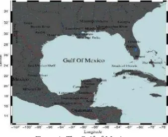
The study area is a region of Gulf of Mexico bounded on the north, northeast and northwest by United States, on the south and southwest by Mexico and on the southeast by Cuba, Ranging from 18.19–30.33˚N in latitude and 80.95–97.78˚W in longitude (see Figure 1).
Figure 1. The Gulf of Mexico.
2.2 Dataset
2.2.1 In-situ data
We validated SSS retrieved from Aquarius instrument on SAC-D satellite with in situ measurements by two COMPS stations from NDBC1(see Figure 2). Most samples in the Gulf of Mexico available at the NDBC are from the northern and eastern shelf regions, with relatively few samples available from offshore waters. The measurements are collected every 30 minutes and mean values over a month are stored (The values are simply sampled in order to obtain monthly maps). We found a good agreement in the validation with R2 of 0.86 and the RMSE of 0.2497. It concludes high consistency between available SSS observations.
Figure 2.Two COMPS stations of in situ data in the Eastern Gulf of Mexico from NDBC. Station 42021-C14- Pasco County Buoy,
Florida with 28.311 N, 83.306 W and station 42022-C12–West Florida Shelf Central Buoy with 27.504 N, 83.741W coordinates.
2.2.2 Satellite data
2.2.2.1
Sea surface salinityAquarius Smoothed SSS data from all three beams for the period from January 2012 to December 2014 were obtained from monthly SSS level 3, version 4 obtained from NASA site (http://neo.sci.gsfc.nasa.gov/). The analysis are applied to SSS products with 0.5˚×0.5˚ spatial resolution. Unfortunately, finer spatial resolution products are not available for Aquarius, mostly because of its sparser space–time sampling (Tzortzi et al., 2013). In version 4 data, static bias adjustment is applied within the sensor were processed to estimate SST using the 11µm band at approximately 4×4 km2 per pixel. They have been used for the 2012-2014 time periods which is obtained from NASA site (https://oceandata.sci.gsfc.nasa.gov).
2.2.2.3
Chlorophyll-a concentrationIn this study, data products of chlorophyll-a concentration (CHLa, mg.m-3) in the surface layer of the Gulf of Mexico region have been obtained from MODIS dataset. This data Comprises of monthly mean sea surface chlorophyll-a maps at 4km resolution. The data set downloaded from http://oceandata.sci.gfsc.nasa.gov. We used version 3 (OCX or OC3) of algorithm for extraction of chlorophyll-a concentration from MODIS data. More details about the retrieving algorithms for CHLa is presented in (O’Reilly et al., 2000).
2.2.2.4
Fresh water fluxFresh water flux or FWF (evaporation minus precipitation) data comprises of two datasets. Precipitation data were taken from the TRMM (Tropical Rainfall Measuring Mission) product. These gridded data have a calendar month temporal resolution and a 0.25˚×0.25˚ spatial resolution. Evaporation were acquired using monthly mean from MODIS Aqua satellite with spatial resolution of 0.1˚.
3. RESULTS AND DISCUSSION
3.1 Spatial distribution of SSS
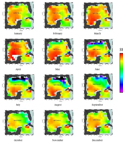
To better comprehension of spatial analysis of SSS variations in the region, the monthly distributions of SSS which obtained by averaging of monthly SSS for three years of study are depicted in Figure 3. On average, the maximum SSSs of about 37psu in the southern Gulf of Mexico are observed in March—May while the minimum SSSs of about 33psu near northern Gulf of Mexico comprise of Mississippi delta, mobile river and Florida coastal waters occur in June-August. We can see that, the SSS value in Southwest is higher than 35.8psu in all of seasons and for Southeast, it is lower mainly because of the low salinity waters of Caribbean Sea. . For all the figures, the maximum rates
of variation in SSS values are for summer. SSS decreases eastward so that eastward currents such as loop current (LC) would bring high-salinity waters from the east to the west, and vice versa. All figures show that north coastal waters in Gulf of Mexico has lower SSS than the other regions. This is mainly
because of Mississippi and Atchafalaya rivers that 70% runoff of Gulf of Mexico is coming from them making waters fresher (Ruoying, 2008).
January February March
April May June
July Augest September
October November December
Figure 3. Monthly climatology of the SSS in the Gulf of Mexico
The International Archives of the Photogrammetry, Remote Sensing and Spatial Information Sciences, Volume XLII-4/W4, 2017 Tehran's Joint ISPRS Conferences of GI Research, SMPR and EOEC 2017, 7–10 October 2017, Tehran, Iran
This contribution has been peer-reviewed.
(a) (b)
(c) (d)
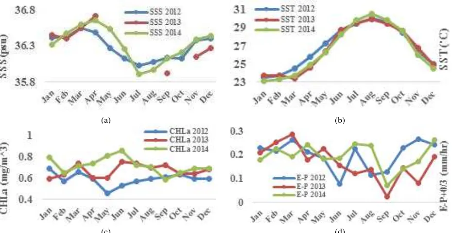
Figure 4. Monthly average variations of (a) SSS, (b) SST, (c) CHLa, and (d) E-P for 2012 to 2014 in the Gulf of Mexico
(a) (b) (c)
Figure 5. Scatter plot between SSS and (a) CHLa, (b) SST, and (c) E-P based on the monthly mean for 2012-2014.
(a) (b) (c)
Figure 6. Spatial distribution of the 3-year averaged (a) SSS, (b), SST, and (c) CHLa in Gulf of Mexico.
3.2 Temporal distribution of SSS
To test the assumption of whether there is a relationship between
time series of these surface ocean parameters based on satellite observations (Figure 4).
Figure 4-a shows the monthly mean SSS in the region from
Generally, the peaks of SSS occur in April except the year 2012 for which the maximum value of SSS observed in March. For all the three years of analysis, SSS initially decreased from spring to summer, and then gradually increased in autumn and winter. The highest spring SSS occurred in the year 2013 with the value of 36.72 psu.
3.3 Relationship between SSS, SST, CHLa and FWF
From Figure 4-b, SST increased from spring to summer and reached its peak in July. The year 2014 had the lowest summer SSS while SST was at its highest value in summer with the value of 30.55˚C. There is a negative relationship between SSS and SST. Figure 5-a shows the scatter plot between the mean SSS and SST in the study region that confirmed the negative and high correlation between SSS and SST with the coefficient of 0.7. From Figure 6-c it is obvious that, high chlorophyll-a concentrations (≥1 mg.m⁻³) occurs inshore and particularly near Major River mouths during the summer seasons of 2012, 2013 and 2014 (Nababan et al., 2011). Figure 4-c shows that there is no significant trend for CHLa concentration variations. The year 2012 had the lowest CHLa in spring, while the minimum value of 0.46 mg.m⁻³ is in May. Figure 4-a and 4-d indicate that the minimum value of SSS and FWF both occur in September and similar to SSS, high rates of FWF occurs in springs which demonstrate the positive correlation between the two variables. This result can be obviously driven from the scatter plot in Figure 5-c with the determination coefficient of 0.22.
4. CONCLUSION
We have presented variability of SSS in the Gulf of Mexico from the Aquarius level3-version4 data set collected from 2012 to 2014. Monitoring of SSS and its trend acquisition by considering physical effective factors from various sources such as SST, Chlorophyll-a Concentrations and evaporation minus precipitation (E-P) have been discussed. From Figure a and 6-b, by considering the spatial distribution based on the annual means, we observed that the variations of SSS and SST with latitude are similar from north coastal waters of Gulf of Mexico to near the tropic of cancer (open sea) and then have opposite trends to south coastal waters. Also it found that there is a negative relationship between the SSS and CHLa in the study region because the high amounts of CHLa occurs inshore where the SSS is lower and vice versa. The maximum values of SSS are in 23.25N and 23.75N latitudes with the value of 38psu and the minimum value occurs in 29.25N. The computation of correlation coefficient has shown that SST and FWF have high influence on SSS variability.
REFERENCES
Bhaskar, T.V.S.U., Chiranjivi, J., 2015. Evaluation of Aquarius Sea Surface Salinity with Argo Sea Surface Salinity in the Tropical Indian Ocean. IEEE Geosci. Remote Sens.
Lett. 12, 1292–1296. salinity and temperature changes in the western Pacific warm pool during 1992–2000. J. Geophys. Res. 107, SRF 3-1–SRF 3-17. doi:10.1029/2001JC000862 Durack, P.J., 2015. Ocean salinity and the global water cycle.
Oceanography 28, 20–31. doi:http://dx.doi.org/ 10.5670/oceanog.2015.03
Fournier, S., Chapron, B., Salisbury, J., Vandemark, D., Reul, N., 2015. Comparison of space borne measurements of Sea Surface Salinity and colored detrital matter in the Amazon plume. J. Geophys. Res. Oceans 120, 3177– 3192. doi:10.1002/ 2014JC010109
Grodsky, S. A., Reverdin, G., Carton, J.A., Coles, V.J., 2014. Year-to-year salinity changes in the Amazon plume: Contrasting 2011 and 2012 Aquarius/SACD and SMOS satellite data. Remote Sens. Environ. 140, 14– 22. doi:doi:10.1016/j.rse.2013.08.033
Ha˚kanson, L., Eklund, J.M., 2010. Relationships between chlorophyll, salinity, phosphorus, and nitrogen in lakes and marine areas. J. Coast. Res., West Palm Beach (Florida) 26, 412–423.
Klemas, V., 2011. Remote sensing of sea surface salinity: an overview with case studies. J. Coast. Res., West Palm Beach (Florida) 27, 830–838.
Lagerloef, G., Colomb, F.R., Le Vine, D., Wentz, F., Yueh, S., Ruf, C., Lilly, J., deCharon, A., C. Swift., Gunn, J., Chao, Y., 2008. The Aquarius/SAC-D Mission: Designed to meet the salinity remote-sensing challenge. Oceanography 21, 68–81.
Le Vine, D., Lagerloef, G., Torrusio, S., 2010. Aquarius and remote sensing of sea surface salinity from space. Proc. IEEE 98, 688–703.
Nababan, B., Muller-Karger, F.E., Hu, C., Biggs, D.C., 2011. Chlorophyll variability in the northeastern Gulf of Mexico. Int. J. Remote Sens. 32, 8373–8391. doi:http://dx.doi.org/10.1080/01431161.2010.542192 O’Reilly, J.E., Maritorena, S., Siegel, D., O’Brien, M.O., 2000.
Ocean color chlorophyll a algorithms for SeaWiFS, OC2, and OC4: Version 4. SeaWiFS Postlaunch Calibration and Validation Analyses, Part 3.
Paytan, A., 2006. Temperature; Salinity; Density; General Ocean Circulation.
Prinn, R.G., 1990. Atmosphere, oceans, and land. EOS 71, 1855– 1857.
Ruoying, H., 2008. Physical Oceanography and Circulation in the Gulf of Mexico Oceanography and Circulation in the Gulf of Mexico. Presented at the Ocean Carbon and Biogeochemistry Scoping Workshop on Terrestrial and Coastal Carbon Fluxes in the Gulf of Mexico, St. Petersburg, FL.
Schmitt, R.W., 1995. The ocean component of the global water cycle. Rev. Geophys. 33, 1395–1409. doi:http://dx.doi.org/10.1029/95RG00184
Tzortzi, E., Josey, S.A., Srokosz, M., Gommenginger, C., 2013. Tropical Atlantic salinity variability: New insights from SMOS. Geophys. Res. Lett. 40, 2143–2147. doi:10.1002/grl.50225
Tzortzi, E., Srokosz, M., Gommenginger, C., Josey, S.A., 2016. Spatial and temporal scales of variability in Tropical Atlantic Sea Surface Salinity from the SMOS and Aquarius satellite missions. Remote Sens. Environ. Vinayachandran, P.N., Nanjundiah, R.S., 2009. Indian Ocean sea
surface salinity variations in a coupled model. Clim. Dyn. 33, 245–263. doi:10.1007/s00382-008-0511-6
The International Archives of the Photogrammetry, Remote Sensing and Spatial Information Sciences, Volume XLII-4/W4, 2017 Tehran's Joint ISPRS Conferences of GI Research, SMPR and EOEC 2017, 7–10 October 2017, Tehran, Iran
This contribution has been peer-reviewed.