Algorithms and Data Structures
© N. Wirth 1985 (Oberon version: August 2004)
Contents Preface
1 Fundamental Data Structures
1.1 Introduction
1.2 The Concept of Data Type 1.3 Primitive Data Types 1.4 Standard Primitive Types
1.4.1 Integer types 1.4.2 The type REAL 1.4.3 The type BOOLEAN 1.4.4 The type CHAR 1.4.5 The type SET 1.5 The Array Structure 1.6 The Record Structure
1.7 Representation of Arrays, Records, and Sets 1.7.1 Representation of Arrays
1.7.2 Representation of Recors 1.7.3 Representation of Sets 1.8 The File (Sequence)
1.8.1 Elementary File Operators 1.8.2 Buffering Sequences
1.8.3 Buffering between Concurrent Processes 1.8.4 Textual Input and Output
1.9 Searching 1.9.1 Linear Search 1.9.2 Binary Search 1.9.3 Table Search
1.9.4 Straight String Search
1.9.5 The Knuth-Morris-Pratt String Search 1.9.6 The Boyer-Moore String Search Exercises
2 Sorting
2.1 Introduction 2.2 Sorting Arrays
2.2.1 Sorting by Straight Insertion 2.2.2 Sorting by Straight Selection 2.2.3 Sorting by Straight Exchange 2.3 Advanced Sorting Methods
2.3.1 Insertion Sort by Diminishing Increment 2.3.2 Tree Sort
2.3.3 Partition Sort 2.3.4 Finding the Median
2.3.5 A Comparison of Array Sorting Methods 2.4 Sorting Sequences
2.4.1 Straight Merging 2.4.2 Natural Merging
2.4.3 Balanced Multiway Merging 2.4.4 Polyphase Sort
3 Recursive Algorithms 3.1 Introduction
3.2 When Not to Use Recursion
3.3 Two Examples of Recursive Programs 3.4 Backtracking Algorithms
3.5 The Eight Queens Problem 3.6 The Stable Marriage Problem 3.7 The Optimal Selection Problem Exercises
4 Dynamic Information Structures
4.1 Recursive Data Types 4.2 Pointers
4.3 Linear Lists
4.3.1 Basic Operations
4.3.2 Ordered Lists and Reorganizing Lists 4.3.3 An Application: Topological Sorting 4.4 Tree Structures
4.4.1 Basic Concepts and Definitions 4.4.2 Basic Operations on Binary Trees 4.4.3 Tree Search and Insertion 4.4.4 Tree Deletion
4.4.5 Analysis of Tree Search and Insertion 4.5 Balanced Trees
4.5.1 Balanced Tree Insertion 4.5.2 Balanced Tree Deletion 4.6 Optimal Search Trees 4.7 B-Trees
4.7.1 Multiway B-Trees 4.7.2 Binary B-Trees 4.8 Priority Search Trees Exercises
5 Key Transformations (Hashing) 5.1 Introduction
5.2 Choice of a Hash Function 5.3 Collision handling
5.4 Analysis of Key Transformation Exercises
Appendices
Preface
In recent years the subject of computer programming has been recognized as a discipline whose mastery is fundamental and crucial to the success of many engineering projects and which is amenable to scientific treatement and presentation. It has advanced from a craft to an academic discipline. The initial outstanding contributions toward this development were made by E.W. Dijkstra and C.A.R. Hoare. Dijkstra's Notes on Structured Programming [1] opened a new view of programming as a scientific subject and intellectual challenge, and it coined the title for a "revolution" in programming. Hoare's
Axiomatic Basis of Computer Programming [2] showed in a lucid manner that programs are amenable to
an exacting analysis based on mathematical reasoning. Both these papers argue convincingly that many programmming errors can be prevented by making programmers aware of the methods and techniques which they hitherto applied intuitively and often unconsciously. These papers focused their attention on the aspects of composition and analysis of programs, or more explicitly, on the structure of algorithms represented by program texts. Yet, it is abundantly clear that a systematic and scientific approach to program construction primarily has a bearing in the case of large, complex programs which involve complicated sets of data. Hence, a methodology of programming is also bound to include all aspects of data structuring. Programs, after all, are concrete formulations of abstract algorithms based on particular representations and structures of data. An outstanding contribution to bring order into the bewildering variety of terminology and concepts on data structures was made by Hoare through his Notes on Data
Structuring [3]. It made clear that decisions about structuring data cannot be made without knowledge of
the algorithms applied to the data and that, vice versa, the structure and choice of algorithms often depend strongly on the structure of the underlying data. In short, the subjects of program composition and data structures are inseparably interwined.
Yet, this book starts with a chapter on data structure for two reasons. First, one has an intuitive feeling that data precede algorithms: you must have some objects before you can perform operations on them. Second, and this is the more immediate reason, this book assumes that the reader is familiar with the basic notions of computer programming. Traditionally and sensibly, however, introductory programming courses concentrate on algorithms operating on relatively simple structures of data. Hence, an introductory chapter on data structures seems appropriate.
Throughout the book, and particularly in Chap. 1, we follow the theory and terminology expounded by Hoare and realized in the programming language Pascal [4]. The essence of this theory is that data in the first instance represent abstractions of real phenomena and are preferably formulated as abstract structures not necessarily realized in common programming languages. In the process of program construction the data representation is gradually refined -- in step with the refinement of the algorithm -- to comply more and more with the constraints imposed by an available programming system [5]. We therefore postulate a number of basic building principles of data structures, called the fundamental structures. It is most important that they are constructs that are known to be quite easily implementable on actual computers, for only in this case can they be considered the true elements of an actual data representation, as the molecules emerging from the final step of refinements of the data description. They are the record, the array (with fixed size), and the set. Not surprisingly, these basic building principles correspond to mathematical notions that are fundamental as well.
A cornerstone of this theory of data structures is the distinction between fundamental and "advanced" structures. The former are the molecules -- themselves built out of atoms -- that are the components of the latter. Variables of a fundamental structure change only their value, but never their structure and never the set of values they can assume. As a consequence, the size of the store they occupy remains constant. "Advanced" structures, however, are characterized by their change of value and structure during the execution of a program. More sophisticated techniques are therefore needed for their implementation. The sequence appears as a hybrid in this classification. It certainly varies its length; but that change in structure is of a trivial nature. Since the sequence plays a truly fundamental role in practically all computer systems, its treatment is included in Chap. 1.
choice of good solutions for a given problem. The partitioning into methods for sorting arrays and methods for sorting files (often called internal and external sorting) exhibits the crucial influence of data representation on the choice of applicable algorithms and on their complexity. The space allocated to sorting would not be so large were it not for the fact that sorting constitutes an ideal vehicle for illustrating so many principles of programming and situations occurring in most other applications. It often seems that one could compose an entire programming course by deleting examples from sorting only.
Another topic that is usually omitted in introductory programming courses but one that plays an important role in the conception of many algorithmic solutions is recursion. Therefore, the third chapter is devoted to recursive algorithms. Recursion is shown to be a generalization of repetition (iteration), and as such it is an important and powerful concept in programming. In many programming tutorials, it is unfortunately exemplified by cases in which simple iteration would suffice. Instead, Chap. 3 concentrates on several examples of problems in which recursion allows for a most natural formulation of a solution, whereas use of iteration would lead to obscure and cumbersome programs. The class of backtracking algorithms emerges as an ideal application of recursion, but the most obvious candidates for the use of recursion are algorithms operating on data whose structure is defined recursively. These cases are treated in the last two chapters, for which the third chapter provides a welcome background.
Chapter 4 deals with dynamic data structures, i.e., with data that change their structure during the execution of the program. It is shown that the recursive data structures are an important subclass of the dynamic structures commonly used. Although a recursive definition is both natural and possible in these cases, it is usually not used in practice. Instead, the mechanism used in its implementation is made evident to the programmer by forcing him to use explicit reference or pointer variables. This book follows this technique and reflects the present state of the art: Chapter 4 is devoted to programming with pointers, to lists, trees and to examples involving even more complicated meshes of data. It presents what is often (and somewhat inappropriately) called list processing. A fair amount of space is devoted to tree organizations, and in particular to search trees. The chapter ends with a presentation of scatter tables, also called "hash" codes, which are oftern preferred to search trees. This provides the possibility of comparing two fundamentally different techniques for a frequently encountered application.
book Systematic Programming [6] provides an ideal background because it is also based on the Pascal notation. The present book was, however, not intended as a manual on the language Pascal; there exist more appropriate texts for this purpose [7].
This book is a condensation -- and at the same time an elaboration -- of several courses on programming taught at the Federal Institute of Technology (ETH) at Zürich. I owe many ideas and views expressed in this book to discussions with my collaborators at ETH. In particular, I wish to thank Mr. H. Sandmayr for his careful reading of the manuscript, and Miss Heidi Theiler and my wife for their care and patience in typing the text. I should also like to mention the stimulating influence provided by meetings of the Working Groups 2.1 and 2.3 of IFIP, and particularly the many memorable arguments I had on these occasions with E. W. Dijkstra and C.A.R. Hoare. Last but not least, ETH generously provided the environment and the computing facilities without which the preparation of this text would have been impossible.
Zürich, Aug. 1975 N. Wirth
1. In Structured Programming. O-.J. Dahl, E.W. Dijkstra, C.A.R. Hoare. F. Genuys, Ed. (New York; Academic Press, 1972), pp. 1-82.
2. In Comm. ACM, 12, No. 10 (1969), 576-83. 3. In Structured Programming, pp. 83-174.
4. N. Wirth. The Programming Language Pascal. Acta Informatica, 1, No. 1 (1971), 35-63.
5. N. Wirth. Program Development by Stepwise Refinement. Comm. ACM, 14, No. 4 (1971), 221-27. 6. N. Wirth. Systematic Programming. (Englewood Cliffs, N.J. Prentice-Hall, Inc., 1973.)
7. K. Jensen and N. Wirth, PASCAL-User Manual and Report. (Berlin, Heidelberg, New York; Springer-Verlag, 1974).
Preface To The 1985 Edition
This new Edition incorporates many revisions of details and several changes of more significant nature. They were all motivated by experiences made in the ten years since the first Edition appeared. Most of the contents and the style of the text, however, have been retained. We briefly summarize the major alterations.
The major change which pervades the entire text concerns the programming language used to express the algorithms. Pascal has been replaced by Modula-2. Although this change is of no fundamental influence to the presentation of the algorithms, the choice is justified by the simpler and more elegant syntactic structures of Modula-2, which often lead to a more lucid representation of an algorithm's structure. Apart from this, it appeared advisable to use a notation that is rapidly gaining acceptance by a wide community, because it is well-suited for the development of large programming systems. Nevertheless, the fact that Pascal is Modula's ancestor is very evident and eases the task of a transition. The syntax of Modula is summarized in the Appendix for easy reference.
As a direct consequence of this change of programming language, Sect. 1.11 on the sequential file structure has been rewritten. Modula-2 does not offer a built-in file type. The revised Sect. 1.11 presents the concept of a sequence as a data structure in a more general manner, and it introduces a set of program modules that incorporate the sequence concept in Modula-2 specifically.
The last part of Chapter 1 is new. It is dedicated to the subject of searching and, starting out with linear and binary search, leads to some recently invented fast string searching algorithms. In this section in particular we use assertions and loop invariants to demonstrate the correctness of the presented algorithms.
The entire fifth chapter of the first Edition has been omitted. It was felt that the subject of compiler construction was somewhat isolated from the preceding chapters and would rather merit a more extensive treatment in its own volume.
Finally, the appearance of the new Edition reflects a development that has profoundly influenced publications in the last ten years: the use of computers and sophisticated algorithms to prepare and automatically typeset documents. This book was edited and laid out by the author with the aid of a Lilith computer and its document editor Lara. Without these tools, not only would the book become more costly, but it would certainly not be finished yet.
Palo Alto, March 1985 N. Wirth
Notation
The following notations, adopted from publications of E.W. Dijkstra, are used in this book.
In logical expressions, the character & denotes conjunction and is pronounced as and. The character ~ denotes negation and is pronounced as not. Boldface A and E are used to denote the universal and existential quantifiers. In the following formulas, the left part is the notation used and defined here in terms of the right part. Note that the left parts avoid the use of the symbol "...", which appeals to the readers intuition.
A
i: m ≤ i < n : Pi ≡ Pm & Pm+1 & ... & Pn-1The Pi are predicates, and the formula asserts that for all indices i ranging from a given value m to, but
excluding a value n, Pi holds.
E
i: m ≤ i < n : Pi ≡ Pm or Pm+1 or ... or Pn-1The Pi are predicates, and the formula asserts that for some indices i ranging from a given value m to, but
excluding a value n, Pi holds.
S
i: m ≤ i < n : xi = xm + xm+1 + ... + xn-1MIN i: m ≤ i < n : xi = minimum(xm , ... , xn-1)
1. Fundamental Data Structures
1.1. Introduction
The modern digital computer was invented and intended as a device that should facilitate and speed up complicated and time-consuming computations. In the majority of applications its capability to store and access large amounts of information plays the dominant part and is considered to be its primary characteristic, and its ability to compute, i.e., to calculate, to perform arithmetic, has in many cases become almost irrelevant.
In all these cases, the large amount of information that is to be processed in some sense represents an abstraction of a part of reality. The information that is available to the computer consists of a selected set of data about the actual problem, namely that set that is considered relevant to the problem at hand, that set from which it is believed that the desired results can be derived. The data represent an abstraction of reality in the sense that certain properties and characteristics of the real objects are ignored because they are peripheral and irrelevant to the particular problem. An abstraction is thereby also a simplification of facts. We may regard a personnel file of an employer as an example. Every employee is represented (abstracted) on this file by a set of data relevant either to the employer or to his accounting procedures. This set may include some identification of the employee, for example, his or her name and salary. But it will most probably not include irrelevant data such as the hair color, weight, and height.
In solving a problem with or without a computer it is necessary to choose an abstraction of reality, i.e., to define a set of data that is to represent the real situation. This choice must be guided by the problem to be solved. Then follows a choice of representation of this information. This choice is guided by the tool that is to solve the problem, i.e., by the facilities offered by the computer. In most cases these two steps are not entirely separable.
The choice of representation of data is often a fairly difficult one, and it is not uniquely determined by the facilities available. It must always be taken in the light of the operations that are to be performed on the data. A good example is the representation of numbers, which are themselves abstractions of properties of objects to be characterized. If addition is the only (or at least the dominant) operation to be performed, then a good way to represent the number n is to write n strokes. The addition rule on this representation is indeed very obvious and simple. The Roman numerals are based on the same principle of simplicity, and the adding rules are similarly straightforward for small numbers. On the other hand, the representation by Arabic numerals requires rules that are far from obvious (for small numbers) and they must be memorized. However, the situation is reversed when we consider either addition of large numbers or multiplication and division. The decomposition of these operations into simpler ones is much easier in the case of representation by Arabic numerals because of their systematic structuring principle that is based on positional weight of the digits.
It is generally known that computers use an internal representation based on binary digits (bits). This representation is unsuitable for human beings because of the usually large number of digits involved, but it is most suitable for electronic circuits because the two values 0 and 1 can be represented conveniently and reliably by the presence or absence of electric currents, electric charge, or magnetic fields.
In this context, the significance of programming languages becomes apparent. A programming language represents an abstract computer capable of interpreting the terms used in this language, which may embody a certain level of abstraction from the objects used by the actual machine. Thus, the programmer who uses such a higher-level language will be freed (and barred) from questions of number representation, if the number is an elementary object in the realm of this language.
The importance of using a language that offers a convenient set of basic abstractions common to most problems of data processing lies mainly in the area of reliability of the resulting programs. It is easier to design a program based on reasoning with familiar notions of numbers, sets, sequences, and repetitions than on bits, storage units, and jumps. Of course, an actual computer represents all data, whether numbers, sets, or sequences, as a large mass of bits. But this is irrelevant to the programmer as long as he or she does not have to worry about the details of representation of the chosen abstractions, and as long as he or she can rest assured that the corresponding representation chosen by the computer (or compiler) is reasonable for the stated purposes.
The closer the abstractions are to a given computer, the easier it is to make a representation choice for the engineer or implementor of the language, and the higher is the probability that a single choice will be suitable for all (or almost all) conceivable applications. This fact sets definite limits on the degree of abstraction from a given real computer. For example, it would not make sense to include geometric objects as basic data items in a general-purpose language, since their proper repesentation will, because of its inherent complexity, be largely dependent on the operations to be applied to these objects. The nature and frequency of these operations will, however, not be known to the designer of a general-purpose language and its compiler, and any choice the designer makes may be inappropriate for some potential applications. In this book these deliberations determine the choice of notation for the description of algorithms and their data. Clearly, we wish to use familiar notions of mathematics, such as numbers, sets, sequences, and so on, rather than computer-dependent entities such as bitstrings. But equally clearly we wish to use a notation for which efficient compilers are known to exist. It is equally unwise to use a closely machine-oriented and machine-dependent language, as it is unhelpful to describe computer programs in an abstract notation that leaves problems of representation widely open. The programming language Pascal had been designed in an attempt to find a compromise between these extremes, and the successor languages Modula-2 and Oberon are the result of decades of experience [1-3]. Oberon retains Pascal's basic concepts and incorporates some improvements and some extensions; it is used throughout this book [1-5]. It has been successfully implemented on several computers, and it has been shown that the notation is sufficiently close to real machines that the chosen features and their representations can be clearly explained. The language is also sufficiently close to other languages, and hence the lessons taught here may equally well be applied in their use.
1.2. The Concept of Data Type
In mathematics it is customary to classify variables according to certain important characteristics. Clear distinctions are made between real, complex, and logical variables or between variables representing individual values, or sets of values, or sets of sets, or between functions, functionals, sets of functions, and so on. This notion of classification is equally if not more important in data processing. We will adhere to the principle that every constant, variable, expression, or function is of a certain type. This type essentially characterizes the set of values to which a constant belongs, or which can be assumed by a variable or expression, or which can be generated by a function.
The primary characteristics of the concept of type that is used throughout this text, and that is embodied in the programming language Oberon, are the following [1-2]:
1. A data type determines the set of values to which a constant belongs, or which may be assumed by a variable or an expression, or which may be generated by an operator or a function.
2. The type of a value denoted by a constant, variable, or expression may be derived from its form or its declaration without the necessity of executing the computational process.
3. Each operator or function expects arguments of a fixed type and yields a result of a fixed type. If an operator admits arguments of several types (e.g., + is used for addition of both integers and real numbers), then the type of the result can be determined from specific language rules.
As a consequence, a compiler may use this information on types to check the legality of various constructs. For example, the mistaken assignment of a Boolean (logical) value to an arithmetic variable may be detected without executing the program. This kind of redundancy in the program text is extremely useful as an aid in the development of programs, and it must be considered as the primary advantage of good high-level languages over machine code (or symbolic assembly code). Evidently, the data will ultimately be represented by a large number of binary digits, irrespective of whether or not the program had initially been conceived in a high-level language using the concept of type or in a typeless assembly code. To the computer, the store is a homogeneous mass of bits without apparent structure. But it is exactly this abstract structure which alone is enabling human programmers to recognize meaning in the monotonous landscape of a computer store.
The theory presented in this book and the programming language Oberon specify certain methods of defining data types. In most cases new data types are defined in terms of previously defined data types. Values of such a type are usually conglomerates of component values of the previously defined constituent types, and they are said to be structured. If there is only one constituent type, that is, if all components are of the same constituent type, then it is known as the base type. The number of distinct values belonging to a type T is called its cardinality. The cardinality provides a measure for the amount of storage needed to represent a variable x of the type T, denoted by x: T.
Since constituent types may again be structured, entire hierarchies of structures may be built up, but, obviously, the ultimate components of a structure are atomic. Therefore, it is necessary that a notation is provided to introduce such primitive, unstructured types as well. A straightforward method is that of
enumerating the values that are to constitute the type. For example in a program concerned with plane
geometric figures, we may introduce a primitive type called shape, whose values may be denoted by the identifiers rectangle, square, ellipse, circle. But apart from such programmer-defined types, there will have to be some standard, predefined types. They usually include numbers and logical values. If an ordering exists among the individual values, then the type is said to be ordered or scalar. In Oberon, all unstructured types are ordered; in the case of explicit enumeration, the values are assumed to be ordered by their enumeration sequence.
With this tool in hand, it is possible to define primitive types and to build conglomerates, structured types up to an arbitrary degree of nesting. In practice, it is not sufficient to have only one general method of combining constituent types into a structure. With due regard to practical problems of representation and use, a general-purpose programming language must offer several methods of structuring. In a mathematical sense, they are equivalent; they differ in the operators available to select components of these structures. The basic structuring methods presented here are the array, the record, the set, and the sequence. More complicated structures are not usually defined as static types, but are instead dynamically generated during the execution of the program, when they may vary in size and shape. Such structures are the subject of Chap. 4 and include lists, rings, trees, and general, finite graphs.
The most important basic operators are comparison and assignment, i.e., the test for equality (and for order in the case of ordered types), and the command to enforce equality. The fundamental difference between these two operations is emphasized by the clear distinction in their denotation throughout this text.
Test for equality: x = y (an expression with value TRUE or FALSE) Assignment to x: x := y (a statement making x equal to y)
These fundamental operators are defined for most data types, but it should be noted that their execution may involve a substantial amount of computational effort, if the data are large and highly structured. For the standard primitive data types, we postulate not only the availability of assignment and comparison, but also a set of operators to create (compute) new values. Thus we introduce the standard operations of arithmetic for numeric types and the elementary operators of propositional logic for logical values.
1.3. Primitive Data Types
A new, primitive type is definable by enumerating the distinct values belonging to it. Such a type is called
an enumeration type. Its definition has the form
TYPE T = (c1, c2, ... , cn)
T is the new type identifier, and the ci are the new constant identifiers.
Examples
TYPE shape = (rectangle, square, ellipse, circle) TYPE color = (red, yellow, green)
TYPE sex = (male, female)
TYPE weekday = (Monday, Tuesday, Wednesday, Thursday, Friday, Saturday, Sunday)
TYPE currency = (franc, mark, pound, dollar, shilling, lira, guilder, krone, ruble, cruzeiro, yen)
TYPE destination = (hell, purgatory, heaven)
TYPE vehicle = (train, bus, automobile, boat, airplane)
TYPE rank = (private, corporal, sergeant, lieutenant, captain, major, colonel, general)
TYPE object = (constant, type, variable, procedure, module) TYPE structure = (array, record, set, sequence)
TYPE condition = (manual, unloaded, parity, skew)
The definition of such types introduces not only a new type identifier, but at the same time the set of identifiers denoting the values of the new type. These identifiers may then be used as constants throughout the program, and they enhance its understandability considerably. If, as an example, we introduce variables s, d, r, and b.
VAR s: sex VAR d: weekday VAR r: rank
then the following assignment statements are possible: s := male
d := Sunday r := major b := TRUE
Evidently, they are considerably more informative than their counterparts s := 1 d := 7 r := 6 b := 2
against the inconsistent use of operators. For example, given the declaration of s above, the statement s := s+1 would be meaningless.
If, however, we recall that enumerations are ordered, then it is sensible to introduce operators that generate the successor and predecessor of their argument. We therefore postulate the following standard operators, which assign to their argument its successor and predecessor respectively:
INC(x) DEC(x)
1.4. Standard Primitive Types
Standard primitive types are those types that are available on most computers as built-in features. They include the whole numbers, the logical truth values, and a set of printable characters. On many computers fractional numbers are also incorporated, together with the standard arithmetic operations. We denote these types by the identifiers
INTEGER, REAL, BOOLEAN, CHAR, SET
1.4.1. Integer types
The type INTEGER comprises a subset of the whole numbers whose size may vary among individual computer systems. If a computer uses n bits to represent an integer in two's complement notation, then the admissible values x must satisfy -2n-1≤ x < 2n-1. It is assumed that all operations on data of this type are
exact and correspond to the ordinary laws of arithmetic, and that the computation will be interrupted in the case of a result lying outside the representable subset. This event is called overflow. The standard operators are the four basic arithmetic operations of addition (+), subtraction (-), multiplication (*), and division (/, DIV).
Whereas the slash denotes ordinary division resulting in a value of type REAL, the operator DIV denotes integer division resulting in a value of type INTEGER. If we define the quotient q = m DIV n and the remainder r = m MOD n, the following relations hold, assuming n > 0:
q*n + r = m and 0 ≤ r < n Examples:
31 DIV 10 = 3 31 MOD 10 = 1 -31 DIV 10 = -4 -31 MOD 10 = 9
We know that dividing by 10n can be achieved by merely shifting the decimal digits n places to the right
and thereby ignoring the lost digits. The same method applies, if numbers are represented in binary instead of decimal form. If two's complement representation is used (as in practically all modern computers), then the shifts implement a division as defined by the above DIV operaton. Moderately sophisticated compilers will therefore represent an operation of the form m DIV 2n or m MOD 2n by a fast shift (or mask) operation.
1.4.2. The type REAL
The type REAL denotes a subset of the real numbers. Whereas arithmetic with operands of the types INTEGER is assumed to yield exact results, arithmetic on values of type REAL is permitted to be inaccurate within the limits of round-off errors caused by computation on a finite number of digits. This is the principal reason for the explicit distinction between the types INTEGER and REAL, as it is made in most programming languages.
Many programming languages do not include an exponentiation operator. The following is an algorithm for the fast computation of y = xn, where n is a non-negative integer.
y := 1.0; i := n;
WHILE i > 0 DO (* x0n = xi * y *)
IF ODD(i) THEN y := y*x END ; x := x*x; i := i DIV 2
END
1.4.3. The type BOOLEAN
The two values of the standard type BOOLEAN are denoted by the identifiers TRUE and FALSE. The Boolean operators are the logical conjunction, disjunction, and negation whose values are defined in Table 1.1. The logical conjunction is denoted by the symbol &, the logical disjunction by OR, and negation by “~”. Note that comparisons are operations yielding a result of type BOOLEAN. Thus, the result of a comparison may be assigned to a variable, or it may be used as an operand of a logical operator in a Boolean expression. For instance, given Boolean variables p and q and integer variables x = 5, y = 8, z = 10, the two assignments
p := x = y
q := (x ≤ y) & (y < z) yield p = FALSE and q = TRUE.
p q p & q p OR q ~p
TRUE TRUE TRUE TRUE FALSE
TRUE FALSE TRUE FALSE FALSE
FALSE TRUE TRUE FALSE TRUE
FALSE FALSE FALSE FALSE TRUE
Table 1.1 Boolean Operators.
The Boolean operators & (AND) and OR have an additional property in most programming languages, which distinguishes them from other dyadic operators. Whereas, for example, the sum x+y is not defined, if either x or y is undefined, the conjunction p&q is defined even if q is undefined, provided that p is FALSE. This conditionality is an important and useful property. The exact definition of & and OR is therefore given by the following equations:
p & q = if p then q else FALSE p OR q = if p then TRUE else q
1.4.4. The type CHAR
The standard type CHAR comprises a set of printable characters. Unfortunately, there is no generally accepted standard character set used on all computer systems. Therefore, the use of the predicate "standard" may in this case be almost misleading; it is to be understood in the sense of "standard on the computer system on which a certain program is to be executed."
The character set defined by the International Standards Organization (ISO), and particularly its American version ASCII (American Standard Code for Information Interchange) is the most widely accepted set. The ASCII set is therefore tabulated in Appendix A. It consists of 95 printable (graphic) characters and 33 control characters, the latter mainly being used in data transmission and for the control of printing equipment.
In order to be able to design algorithms involving characters (i.e., values of type CHAR) that are system independent, we should like to be able to assume certain minimal properties of character sets, namely: 1. The type CHAR contains the 26 capital Latin letters, the 26 lower-case letters, the 10 decimal digits,
("A" ≤ x) & (x ≤ "Z") implies that x is a capital letter ("a" ≤ x) & (x ≤ "z") implies that x is a lower-case letter ("0" ≤ x) & (x ≤ "9") implies that x is a decimal digit
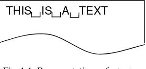
3. The type CHAR contains a non-printing, blank character and a line-end character that may be used as separators.
Fig. 1.1. Representations of a text
The availability of two standard type transfer functions between the types CHAR and INTEGER is particularly important in the quest to write programs in a machine independent form. We will call them ORD(ch), denoting the ordinal number of ch in the character set, and CHR(i), denoting the character with ordinal number i. Thus, CHR is the inverse function of ORD, and vice versa, that is,
ORD(CHR(i)) = i (if CHR(i) is defined) CHR(ORD(c)) = c
Furthermore, we postulate a standard function CAP(ch). Its value is defined as the capital letter corresponding to ch, provided ch is a letter.
ch is a lower-case letter implies that CAP(ch) = corresponding capital letter ch is a capital letter implies that CAP(ch) = ch
1.4.5. The type SET
The type SET denotes sets whose elements are integers in the range 0 to a small number, typically 31 or 63. Given, for example, variables
VAR r, s, t: SET possible assignments are
r := {5}; s := {x, y .. z}; t := {}
Here, the value assigned to r is the singleton set consisting of the single element 5; to t is assigned the empty set, and to s the elements x, y, y+1, … , z-1, z.
The following elementary operators are defined on variables of type SET: * set intersection
+ set union - set difference
/ symmetric set difference IN set membership
Constructing the intersection or the union of two sets is often called set multiplication or set addition, respectively; the priorities of the set operators are defined accordingly, with the intersection operator having priority over the union and difference operators, which in turn have priority over the membership operator, which is classified as a relational operator. Following are examples of set expressions and their fully parenthesized equivalents:
r * s + t = (r*s) + t r - s * t = r - (s*t) r - s + t = (r-s) + t
r + s / t = r + (s/t) x IN s + t = x IN (s+t)
1.5. The Array Structure
The array is probably the most widely used data structure; in some languages it is even the only one available. An array consists of components which are all of the same type, called its base type; it is therefore called a homogeneous structure. The array is a random-access structure, because all components can be selected at random and are equally quickly accessible. In order to denote an individual component, the name of the entire structure is augmented by the index selecting the component. This index is to be an integer between 0 and n-1, where n is the number of elements, the size, of the array.
TYPE T = ARRAY n OF T0 Examples
TYPE Row = ARRAY 4 OF REAL TYPE Card = ARRAY 80 OF CHAR TYPE Name = ARRAY 32 OF CHAR A particular value of a variable
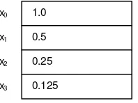
VAR x: Row
with all components satisfying the equation xi = 2-i, may be visualized as shown in Fig. 1.2.
Fig. 1.2 Array of type Row with xi = 2-i
An individual component of an array can be selected by an index. Given an array variable x, we denote an array selector by the array name followed by the respective component's index i, and we write xi or x[i].
Because of the first, conventional notation, a component of an array component is therefore also called a
subscripted variable.
The common way of operating with arrays, particularly with large arrays, is to selectively update single components rather than to construct entirely new structured values. This is expressed by considering an array variable as an array of component variables and by permitting assignments to selected components, such as for example x[i] := 0.125. Although selective updating causes only a single component value to change, from a conceptual point of view we must regard the entire composite value as having changed too. The fact that array indices, i.e., names of array components, are integers, has a most important consequence: indices may be computed. A general index expression may be substituted in place of an index constant; this expression is to be evaluated, and the result identifies the selected component. This generality not only provides a most significant and powerful programming facility, but at the same time it also gives rise to one of the most frequently encountered programming mistakes: The resulting value may be outside the interval specified as the range of indices of the array. We will assume that decent computing systems provide a warning in the case of such a mistaken access to a non-existent array component. The cardinality of a structured type, i. e. the number of values belonging to this type, is the product of the cardinality of its components. Since all components of an array type T are of the same base type T0, we obtain
card(T) = card(T0)n
1.0 x0
0.5 x1
0.25 x2
Constituents of array types may themselves be structured. An array variable whose components are again arrays is called a matrix. For example,
M: ARRAY 10 OF Row
is an array consisting of ten components (rows), each constisting of four components of type REAL, and is called a 10 × 4 matrix with real components. Selectors may be concatenated accordingly, such that Mij and
M[i][j] denote the j th component of row Mi, which is the i th component of M. This is usually abbreviated
as M[i, j] and in the same spirit the declaration M: ARRAY 10 OF ARRAY 4 OF REAL can be written more concisely as
M: ARRAY 10, 4 OF REAL.
If a certain operation has to be performed on all components of an array or on adjacent components of a section of the array, then this fact may conveniently be emphasized by using the FOR satement, as shown in the following examples for computing the sum and for finding the maximal element of an array declared as
VAR a: ARRAY N OF INTEGER sum := 0;
FOR i := 0 TO N-1 DO sum := a[i] + sum END k := 0; max := a[0];
FOR i := 1 TO N-1 DO
IF max < a[i] THEN k := i; max := a[k] END END.
In a further example, assume that a fraction f is represented in its decimal form with k-1 digits, i.e., by an array d such that
f =
S
i : 0 ≤ i < k: di * 10-i orf = d0 + 10*d1 + 100*d2 + … + dk-1*10k-1
Now assume that we wish to divide f by 2. This is done by repeating the familiar division operation for all k-1 digits di, starting with i=1. It consists of dividing each digit by 2 taking into account a possible carry
from the previous position, and of retaining a possible remainder r for the next position: r := 10*r +d[i]; d[i] := r DIV 2; r := r MOD 2
This algorithm is used to compute a table of negative powers of 2. The repetition of halving to compute 2-1, 2-2, ... , 2-N is again appropriately expressed by a FOR statement, thus leading to a nesting of two FOR statements.
PROCEDURE Power(VAR W: Texts.Writer; N: INTEGER); (*compute decimal representation of negative powers of 2*) VAR i, k, r: INTEGER;
d: ARRAY N OF INTEGER; BEGIN
FOR k := 0 TO N-1 DO Texts.Write(W, "."); r := 0; FOR i := 0 TO k-1 DO
r := 10*r + d[i]; d[i] := r DIV 2; r := r MOD 2; Texts.Write(W, CHR(d[i] + ORD("0"))) END ;
d[k] := 5; Texts.Write(W, "5"); Texts.WriteLn(W) END
END Power.
.5 .25 .125 .0625 .03125 .015625 .0078125 .00390625 .001953125 .0009765625
1.6. The Record Structure
The most general method to obtain structured types is to join elements of arbitrary types, that are possibly themselves structured types, into a compound. Examples from mathematics are complex numbers, composed of two real numbers, and coordinates of points, composed of two or more numbers according to the dimensionality of the space spanned by the coordinate system. An example from data processing is describing people by a few relevant characteristics, such as their first and last names, their date of birth, sex, and marital status.
In mathematics such a compound type is the Cartesian product of its constituent types. This stems from the fact that the set of values defined by this compound type consists of all possible combinations of values, taken one from each set defined by each constituent type. Thus, the number of such combinations, also called n-tuples, is the product of the number of elements in each constituent set, that is, the cardinality of the compound type is the product of the cardinalities of the constituent types.
In data processing, composite types, such as descriptions of persons or objects, usually occur in files or data banks and record the relevant characteristics of a person or object. The word record has therefore become widely accepted to describe a compound of data of this nature, and we adopt this nomenclature in preference to the term Cartesian product. In general, a record type T with components of the types T1, T2, ... , Tn is defined as follows:
TYPE T = RECORD s1: T1; s2: T2; ... sn: Tn END card(T) = card(T1) * card(T2) * ... * card(Tn)
Examples
TYPE Complex = RECORD re, im: REAL END
TYPE Date = RECORD day, month, year: INTEGER END TYPE Person = RECORD name, firstname: Name;
birthdate: Date; sex: (male, female);
marstatus: (single, married, widowed, divorced) END
We may visualize particular, record-structured values of, for example, the variables z: Complex
Fig. 1.3. Records of type Complex, Date, and Person
The identifiers s1, s2, ... , sn introduced by a record type definition are the names given to the individual components of variables of that type. As components of records are called fields, the names are field
identifiers. They are used in record selectors applied to record structured variables. Given a variable x: T,
its i-th field is denoted by x.si. Selective updating of x is achieved by using the same selector denotation on the left side in an assignment statement:
x.si := e
where e is a value (expression) of type Ti. Given, for example, the record variables z, d, and p declared above, the following are selectors of components:
z.im (of type REAL)
d.month (of type INTEGER)
p.name (of type Name)
p.birthdate (of type Date) p.birthdate.day (of type INTEGER)
The example of the type Person shows that a constituent of a record type may itself be structured. Thus, selectors may be concatenated. Naturally, different structuring types may also be used in a nested fashion. For example, the i-th component of an array a being a component of a record variable r is denoted by r.a[i], and the component with the selector name s of the i-th record structured component of the array a is denoted by a[i].s.
It is a characteristic of the Cartesian product that it contains all combinations of elements of the constituent types. But it must be noted that in practical applications not all of them may be meaningful. For instance, the type Date as defined above includes the 31st April as well as the 29th February 1985, which are both dates that never occurred. Thus, the definition of this type does not mirror the actual situation entirely correctly; but it is close enough for practical purposes, and it is the responsibility of the programmer to ensure that meaningless values never occur during the execution of a program.
The following short excerpt from a program shows the use of record variables. Its purpose is to count the number of persons represented by the array variable family that are both female and single:
VAR count: INTEGER;
family: ARRAY N OF Person; count := 0;
FOR i := 0 TO N-1 DO
IF (family[i].sex = female) & (family[i].marstatus = single) THEN INC(count) END END
The record structure and the array structure have the common property that both are random-access
structures. The record is more general in the sense that there is no requirement that all constituent types must be identical. In turn, the array offers greater flexibility by allowing its component selectors to be computable values (expressions), whereas the selectors of record components are field identifiers declared in the record type definition.
1.0 -1.0 Complex z
1 4 Date d
1973
SMITH JOHN Person p
male
18 1 1986
1.7. Representation Of Arrays, Records, And Sets
The essence of the use of abstractions in programming is that a program may be conceived, understood, and verified on the basis of the laws governing the abstractions, and that it is not necessary to have further insight and knowledge about the ways in which the abstractions are implemented and represented in a particular computer. Nevertheless, it is essential for a professional programmer to have an understanding of widely used techniques for representing the basic concepts of programming abstractions, such as the fundamental data structures. It is helpful insofar as it might enable the programmer to make sensible decisions about program and data design in the light not only of the abstract properties of structures, but also of their realizations on actual computers, taking into account a computer's particular capabilities and limitations.
The problem of data representation is that of mapping the abstract structure onto a computer store. Computer stores are - in a first approximation - arrays of individual storage cells called bytes. They are understood to be groups of 8 bits. The indices of the bytes are called addresses.
VAR store: ARRAY StoreSize OF BYTE
The basic types are represented by a small number of bytes, typically 2, 4, or 8. Computers are designed to transfer internally such small numbers (possibly 1) of contiguous bytes concurrently, ”in parallel”. The unit transferable concurrently is called a word.
1.7.1. Representation of Arrays
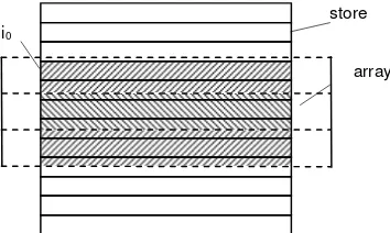
A representation of an array structure is a mapping of the (abstract) array with components of type T onto the store which is an array with components of type BYTE. The array should be mapped in such a way that the computation of addresses of array components is as simple (and therefore as efficient) as possible. The address i of the j-th array component is computed by the linear mapping function
i = i0 + j*s
where i0 is the address of the first component, and s is the number of words that a component occupies.
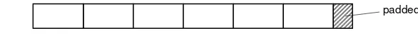
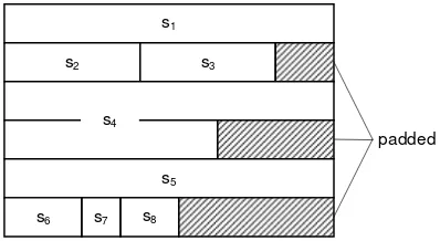
Assuming that the word is the smallest individually transferable unit of store, it is evidently highly desirable that s be a whole number, the simplest case being s = 1. If s is not a whole number (and this is the normal case), then s is usually rounded up to the next larger integer S. Each array component then occupies S words, whereby S-s words are left unused (see Figs. 1.5 and 1.6). Rounding up of the number of words needed to the next whole number is called padding. The storage utilization factor u is the quotient of the minimal amounts of storage needed to represent a structure and of the amount actually used:
u = s / (s rounded up to nearest integer)
Fig. 1.5. Mapping an array onto a store
unused s=2.3 S=3 i0
store
Fig. 1.6. Padded representation of a record
Since an implementor has to aim for a storage utilization as close to 1 as possible, and since accessing parts of words is a cumbersome and relatively inefficient process, he or she must compromise. The following considerations are relevant:
1. Padding decreases storage utilization.
2. Omission of padding may necessitate inefficient partial word access.
3. Partial word access may cause the code (compiled program) to expand and therefore to counteract the gain obtained by omission of padding.
In fact, considerations 2 and 3 are usually so dominant that compilers always use padding automatically. We notice that the utilization factor is always u > 0.5, if s > 0.5. However, if s ≤ 0.5, the utilization factor may be significantly increased by putting more than one array component into each word. This technique is called packing. If n components are packed into a word, the utilization factor is (see Fig. 1.7)
u = n*s / (n*s rounded up to nearest integer)
Fig. 1.7. Packing 6 components into one word
Access to the i-th component of a packed array involves the computation of the word address j in which the desired component is located, and it involves the computation of the respective component position k within the word.
j = i DIV n k = i MOD n
In most programming languages the programmer is given no control over the representation of the abstract data structures. However, it should be possible to indicate the desirability of packing at least in those cases in which more than one component would fit into a single word, i.e., when a gain of storage economy by a factor of 2 and more could be achieved. We propose the convention to indicate the desirability of packing by prefixing the symbol ARRAY (or RECORD) in the declaration by the symbol PACKED.
1.7.2. Representation of Records
Records are mapped onto a computer store by simply juxtaposing their components. The address of a component (field) ri relative to the origin address of the record r is called the field's offset ki. It is computed
as
ki = s1 + s2 + ... + si-1 k0 = 0
where sj is the size (in words) of the j-th component. We now realize that the fact that all components of an
array are of equal type has the welcome consequence that ki = i×s. The generality of the record structure
does unfortunately not allow such a simple, linear function for offset address computation, and it is therefore the very reason for the requirement that record components be selectable only by fixed identifiers. This restriction has the desirable benefit that the respective offsets are known at compile time. The resulting greater efficiency of record field access is well-known.
The technique of packing may be beneficial, if several record components can be fitted into a single storage word (see Fig. 1.8). Since offsets are computable by the compiler, the offset of a field packed within a word may also be determined by the compiler. This means that on many computers packing of records causes a deterioration in access efficiency considerably smaller than that caused by the packing of arrays.
Fig. 1.8. Representation of a packed record
1.7.3. Representation of Sets
A set s is conveniently represented in a computer store by its characteristic function C(s). This is an array of logical values whose ith component has the meaning “i is present in s”. As an example, the set of small integers s = {2, 3, 5, 7, 11, 13} is represented by the sequence of bits, by a bitstring:
C(s) = (… 0010100010101100)
The representation of sets by their characteristic function has the advantage that the operations of computing the union, intersection, and difference of two sets may be implemented as elementary logical operations. The following equivalences, which hold for all elements i of the base type of the sets x and y, relate logical operations with operations on sets:
i IN (x+y) = (i IN x) OR (i IN y) i IN (x*y) = (i IN x) & (i IN y) i IN (x-y) = (i IN x) & ~(i IN y)
These logical operations are available on all digital computers, and moreover they operate concurrently on all corresponding elements (bits) of a word. It therefore appears that in order to be able to implement the basic set operations in an efficient manner, sets must be represented in a small, fixed number of words upon which not only the basic logical operations, but also those of shifting are available. Testing for membership is then implemented by a single shift and a subsequent (sign) bit test operation. As a consequence, a test of the form x IN {c1, c2, ... , cn} can be implemented considerably more efficiently than the equivalent Boolean expression
(x = c1) OR (x = c2) OR ... OR (x = cn)
A corollary is that the set structure should be used only for small integers as elements, the largest one being the wordlength of the underlying computer (minus 1).
1.8. The File or Sequence
Another elementary structuring method is the sequence. A sequence is typically a homogeneous structure like the array. That is, all its elements are of the same type, the base type of the sequence. We shall denote a sequence s with n elements by
s = <s0, s1, s2, ... , sn-1>
n is called the length of the sequence. This structure looks exactly like the array. The essential difference is that in the case of the array the number of elements is fixed by the array's declaration, whereas for the sequence it is left open. This implies that it may vary during execution of the program. Although every sequence has at any time a specific, finite length, we must consider the cardinality of a sequence type as infinite, because there is no fixed limit to the potential length of sequence variables.
A direct consequence of the variable length of sequences is the impossibility to allocate a fixed amount of storage to sequence variables. Instead, storage has to be allocated during program execution, namely whenever the sequence grows. Perhaps storage can be reclaimed when the sequence shrinks. In any case, a
s1
s2 s3
s5
s6 s7 s8
s4
dynamic storage allocation scheme must be employed. All structures with variable size share this property, which is so essential that we classify them as advanced structures in contrast to the fundamental structures discussed so far.
What, then, causes us to place the discussion of sequences in this chapter on fundamental structures? The primary reason is that the storage management strategy is sufficiently simple for sequences (in contrast to other advanced structures), if we enforce a certain discipline in the use of sequences. In fact, under this proviso the handling of storage can safely be delegated to a machanism that can be guaranteed to be reasonably effective. The secondary reason is that sequences are indeed ubiquitous in all computer applications. This structure is prevalent in all cases where different kinds of storage media are involved, i.e. where data are to be moved from one medium to another, such as from disk or tape to primary store or vice-versa.
The discipline mentioned is the restraint to use sequential access only. By this we mean that a sequence is inspected by strictly proceeding from one element to its immediate successor, and that it is generated by repeatedly appending an element at its end. The immediate consequence is that elements are not directly
accessible, with the exception of the one element which currently is up for inspection. It is this accessing
discipline which fundamentally distinguishes sequences from arrays. As we shall see in Chapter 2, the influence of an access discipline on programs is profound.
The advantage of adhering to sequential access which, after all, is a serious restriction, is the relative simplicity of needed storage management. But even more important is the possibility to use effective buffering techniques when moving data to or from secondary storage devices. Sequential access allows us to feed streams of data through pipes between the different media. Buffering implies the collection of sections of a stream in a buffer, and the subsequent shipment of the whole buffer content once the buffer is filled. This results in very significantly more effective use of secondary storage. Given sequential access only, the buffering mechanism is reasonably straightforward for all sequences and all media. It can therefore safely be built into a system for general use, and the programmer need not be burdened by incorporating it in the program. Such a system is usually called a file system, because the high-volume, sequential access devices are used for permanent storage of (persistent) data, and they retain them even when the computer is switched off. The unit of data on these media is commonly called (sequential) file. Here we will use the term file as synonym to sequence.
There exist certain storage media in which the sequential access is indeed the only possible one. Among them are evidently all kinds of tapes. But even on magnetic disks each recording track constitutes a storage facility allowing only sequential access. Strictly sequential access is the primary characteristic of every mechanically moving device and of some other ones as well.
It follows that it is appropriate to distinguish between the data structure, the sequence, on one hand, and
the mechanism to access elements on the other hand. The former is declared as a data structure, the latter
typically by the introduction of a record with associated operators, or, according to more modern terminology, by a rider object. The distinction between data and mechanism declarations is also useful in view of the fact that several access points may exist concurrently on one and the same sequence, each one representing a sequential access at a (possibly) different location.
We summarize the essence of the foregoing as follows:
1. Arrays and records are random access structures. They are used when located in primary, random-access store.
2. Sequences are used to access data on secondary, sequential-access stores, such as disks and tapes. 3. We distinguish between the declaration of a sequence variable, and that of an access mechanism located
at a certain position within the seqence.
1.8.1 Elementary File Operators
Sequences, files, are typically large, dynamic data structures stored on a secondary storage device. Such a device retains the data even if a program is terminated, or a computer is switched off. Therefore the introduction of a file variable is a complex operation connecting the data on the external device with the file variable in the program. We therefore define the type File in a separate module, whose definition specifies the type together with its operators. We call this module Files and postulate that a sequence or file variable must be explicitly initialized (opened) by calling an appropriate operator or function:
VAR f: File f := Open(name)
where name identifies the file as recorded on the persistent data carrier. Some systems distinguish between opening an existing file and opening a new file:
f := Old(name) f := New(name)
The disconnection between secondary storage and the file variable then must also be explicitly requested by, for example, a call of Close(f).
Evidently, the set of operators must contain an operator for generating (writing) and one for inspecting (reading) a sequence. We postulate that these operations apply not to a file directly, but to an object called a
rider, which itself is connected with a file (sequence), and which implements a certain access mechanism.
The sequential access discipline is guaranteed by a restrictive set of access operators (procedures).
A sequence is generated by appending elements at its end after having placed a rider on the file. Assuming the declaration
VAR r: Rider
we position the rider r on the file f by the statement Set(r, f, pos)
where pos = 0 designates the beginning of the file (sequence). A typical pattern for generating the sequence is:
WHILE more DO compute next element x; Write(r, x) END
A sequence is inspected by first positioning a rider as shown above, and then proceeding from element to element. A typical pattern for reading a sequence is:
Read(r, x);
WHILE ~r.eof DO process element x; Read(r, x) END
Evidently, a certain position is always associated with every rider. It is denoted by r.pos. Furthermore, we postulate that a rider contain a predicate (flag) r.eof indicating whether a preceding read operation had reached the sequence’s end. We can now postulate and describe informally the following set of primitive operators:
1a. New(f, name) defines f to be the empty sequence.
1b. Old(f, name) defines f to be the sequence persistently stored with given name. 2. Set(r, f, pos) associate rider r with sequence f, and place it at position pos.
3. Write(r, x) place element with value x in the sequence designated by rider r, and advance. 4. Read(r, x) assign to x the value of the element designated by rider r, and advance. 5. Close(f) registers the written file f in the persistent store (flush buffers).
Note: Writing an element in a sequence is often a complex operation. However, mostly, files are created by appending elements at the end.
characteristics of the primitive sequence operators, independently on how the sequences are represented in store.
The operators are presented in terms of conventional procedures. This collection of definitions of types, variables, and procedure headings (signatures) is called a definition. We assume that we are to deal with sequences of characters, i.e. text files whose elements are of type CHAR. The declarations of File and
Rider are good examples of an application of record structures because, in addition to the field denoting the
array which represents the data, further fields are required to denote the current length and position, i.e. the state of the rider.
DEFINITION Files;
TYPE File; (*sequence of characters*) Rider = RECORD eof: BOOLEAN END ;
PROCEDURE New(VAR name: ARRAY OF CHAR): File; PROCEDURE Old(VAR name: ARRAY OF CHAR): File; PROCEDURE Close(VAR f: File);
PROCEDURE Set(VAR r: Rider; VAR f: File; pos: INTEGER); PROCEDURE Write (VAR r: Rider; ch: CHAR);
PROCEDURE Read (VAR r: Rider; VAR ch: CHAR); END Files.
A definition represents an abstraction. Here we are given the two data types, File and Rider, together with
their operations, but without further details revealing their actual representation in store. Of the operators, declared as procedures, we see their headings only. This hiding of the details of implementation is intentional. The concept is called information hiding. About riders we only learn that there is a property called eof. This flag is set, if a read operation reaches the end of the file. The rider’s position is invisible, and hence the rider’s invariant cannot be falsified by direct access. The invariant expresses the fact that the position always lies within the limits given by the associated sequence. The invariant is established by procedure Set, and required and maintained by procedures Read and Write.
The statements that implement the procedures and further, internal details of the data types, are sepecified in a construct called module. Many representations of data and implementations of procedures are possible. We chose the following as a simple example (with fixed maximal file length):
MODULE Files;
CONST MaxLength = 4096;
TYPE File = POINTER TO RECORD len: INTEGER;
a: ARRAY MaxLength OF CHAR END ;
Rider = RECORD (* 0 <= pos <= s.len <= Max Length *) f: File; pos: INTEGER; eof: BOOLEAN
END ;
PROCEDURE New(name: ARRAY OF CHAR): File; VAR f: File;
BEGIN NEW(f); f.length := 0; f.eof := FALSE; (*directory operation omitted*) RETURN f
END New;
PROCEDURE Old(name: ARRAY OF CHAR): File; VAR f: File;
BEGIN NEW(f); f.eof := FALSE; (*directory lookup omitted*) RETURN f
END New;
PROCEDURE Close(VAR f: File); BEGIN
PROCEDURE Set(VAR r: Rider; f: File; pos: INTEGER); BEGIN (*assume f # NIL*) r.f := f; r.eof := FALSE;
IF pos >= 0 THEN
IF pos <= s.len THEN r.pos := pos ELSE r.pos := s.len END ELSE r.pos := 0
END END Set;
PROCEDURE Write(VAR r: Rider; ch: CHAR); BEGIN
IF (r.pos <= r.s.len) & (r.pos < MaxLength) THEN r.a[r.pos] := ch; INC(r.pos);
IF r.pos = r.f.len THEN INC(r.f.len) END ELSE r.eof := TRUE
END END Write;
PROCEDURE Read(VAR r: Rider; VAR ch: CHAR); BEGIN
IF r.pos < r.f.length THEN ch := r.f.a[r.pos]; INC(r.pos) ELSE r.eof := TRUE END END Read;
END Files.
Note that in this example the maximum length that sequences may reach is an arbitrary constant. Should a program cause a sequence to become longer, then this would not be a mistake of the program, but an inadequacy of this implementation. On the other hand, a read operation proceeding beyond the current end of the sequence would indeed be the program's mistake. Here, the flag r.eof is also used by the write operation to indicate that it was not possible to perform it. Hence, ~r.eof is a precondition for both Read and Write.
1.8.2. Buffering sequences
When data are transferred to or from a secondary storage device, the individual bits are transferred as a stream. Usually, a device imposes strict timing constraints upon the transmission. For example, if data are written on a tape, the tape moves at a fixed speed and requires the data to be fed at a fixed rate. When the source ceases, the tape movement is switched off and speed decreases quickly, but not instantaneously. Thus a gap is left between the data transmitted and the data to follow at a later time. In order to achieve a high density of data, the number of gaps ought to be kept small, and therefore data are transmitted in relatively large blocks once the tape is moving. Similar conditions hold for magnetic disks, where the data are allocated on tracks with a fixed number of blocks of fixed size, the so-called block size. In fact, a disk should be regarded as an array of blocks, each block being read or written as a whole, containing typically 2k bytes with k = 8, 9, … 12.
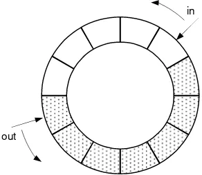
Our programs, however, do not observe any such timing constraints. In order to allow them to ignore the constraints, the data to be transferred are buffered. They are collected in a buffer variable (in main store) and transferred when a sufficient amount of data is accumulated to form a block of the required size. The buffer’s client has access only via the two procedures deposit and fetch.
DEFINITION Buffer;
PROCEDURE deposit(x: CHAR); PROCEDURE fetch(VAR x: CHAR); END Buffer.
Buffering has an additional advantage in allowing the process which generates (receives) data to proceed concurrently with the device that writes (reads) the data from (to) the buffer. In fact, it is convenient to regard the device as a process itself which merely copies data streams. The buffer's purpose is to provide a certain degree of decoupling between the two processes, which we shall call the producer and the
consumer. If, for example, the consumer is slow at a certain moment, it may catch up with the producer
effect, if the rates of producer and consumer are about the same on the average, but fluctuate at times. The degree of decoupling grows wi