ZERO GRAVITY OF A JET
EMERGING FROM A SLIT
L.H. Wiryanto
Abstract. A jet formed as a fluid flows through a slit between two rectangle walls is
presented as a model for the case of zero gravity. The analytical solution is obtained by using hodograph transformation for the slope of the free boundaries of the jet. This is then used to determine the relation between the coordinates of the separation point of the vertical wall and the asymptotic angle of the jet.
1. INTRODUCTION
A 2-D steady flow passing through a slit and producing a jet is considered. At the beginning the fluid occupies a domain bounded by two rectangular walls, and a slit is built by shifting one of the walls such that a jet is formed as the fluid flows through the slit. The problem here is to determine the profile of the jet which is a stream between two free boundaries.
In solving of the problem we assume that the fluid flow is irrotational and the fluid is inviscid and incompressible. Moreover, we simplify the model by considering the influence of gravity relative to inertia is negligible. Physically, the jet asymp-totes downstream to a uniform stream, which is straight and declines downward at the same unique angle, to be determined. An exact solution can be obtained via a hodograph transformation in determining the slope of both free boundaries of the jet, since the speed of the fluid flow is constant along the free boundaries. The similar works can be seen in Dias & Tuck [1] for a flow over a vertical weir, and further generalized by Wiryanto [5] for various angles of the weir. Other references
Received 4 August 2005, Revised 12 October 2005, Accepted 18 October 2005.
2000 Mathematics Subject Classification: 76B07.
Key words and Phrases: Zero gravity, jet emerging from a slit, hodograph transformation.
In this paper we solve the problem for the fluid domain which is rectangle and involving two separation points, as the change of the boundary from solid to free surface. When we choose one of the separation point as the reference of coor-dinates, the coordinates of the other point should be an input parameter. However the domain transformation requires the artificial parameter rather than physical coordinates. Therefore, we determine the relation between both parameters, and the asymptotic angle of the jet.
In discussing the problem, we first formulate the model in artificial variables. This produces a boundary value problem of Laplace equation presented in Section 2. The analytical solution of the slope of the free boundaries of the jet is obtained by introducing an analytic complex function and applying Cauchy theorem. We discuss the solution in Section 3. This is then followed by discussing the result in Section 4. Some numerical calculations are used to reformulate the result in physical domain.
2. MATHEMATICAL FORMULATION
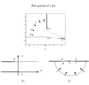
Let us consider the steady two-dimensional fluid flow such as illustrated in Figure 1a. Two walls, given in bold line, bound the fluid, and make a slit at the bottom corner by shifting one of the walls. Here we assume that the volume of the fluid is infinity by expressing no boundaries at the left and above. Therefore, the fluxQof the flow has less velocity for the fluid far from the slit.
Without loss of generality we choose the bottom wall as a fixed boundary and also as the reference of the horizontal axis. The vertical axis is chosen rectangle to the horizontal one and passing the separation pointAof the bottom wall. The vertical wall is shifted upward and either right or left so that the coordinates of the separation point B of this wall is (L, W).
From the assumption for the fluid and the flow, we can present the stream in a complex potential f = φ+iψ, which corresponds to the complex velocity df /dz = u−iv. We other define the fluid flow domain in a physical plane as z =x+iy. For convenience, we work in non-dimensional variables by taking Q as the unit flux and W as the unit length, and we choose φ = 0, ψ = 0 at the separation pointA. Therefore, the f-plane is a strip with width 1, also the width of the slit. Now, our task is to solve the boundary value problem
∇2f = 0
in the flow domain, subject to the dynamics condition expressed by Bernoulli’s equation
Figure 1: (a) shows a schematic diagram of the non-dimensional physicalz-plane, whilst (b)and (c) show the complex potential f-plane and the artificial ζ-plane respectively.
along the free boundaries for zero gravity, and kinematics condition
∂φ
∂~n = 0 (2)
where~nis a normal vector of the boundaries.
In determiningφ(orψ), we introduce a hodograph variable Ω =τ−iθhaving a relationship
df dz =e
Ω (3)
and an artificial planeζ=ξ+iηsatisfying
f =−π1 logζ. (4)
is now to determine Ω satisfying
Condition (5) is obtained by substituting (3) to (1), and condition (6) expresses the kinematics (2) along the vertical and horizontal walls.
3. ANALYTICAL SOLUTION
In this section, we solve analytically Ω(ξ) satisfying the boundary value prob-lem derived in the previous section, more specific the value of θ along the free boundariesξb< ξ <1. To do so, we define an analytic complex function, namely
χ(ζ) = Ω(ζ)(1−ζ)−1/2
(ζ+ξb)−1/2 (7)
The square root behavior represents the flow near the separation pointsζ= 1 and ζ =ξb havingθ=O(ζ−1/2), see Wiryanto [4]. The function (7) is then expressed
along the realζ-axis by substituting (5) and (6), giving
χ(ξ) = fore, Cauchy’s integral formula can be applied toχon a path consisting of the real ζ-axis, a semi-circular at|ζ|=∞in the lower half plane, and a circle of vanishing radius about the pointζ∗
. This is then taken Im(ζ∗
The tangential θ of the streamline along the free boundaries can be deter-mined by substituting (8) into both sides of (9). For anyξ∗
in (ξb,1), the left hand
side of (9) reduces to −iθ/p(1−ξ∗)(ξ∗
(9) contains a complex integrand in which the imaginary part is equated to the
The integral can be determined, using antiderivative
Z dx
The result (11) is firstly checked for the value ofθnear the separation pointB. In the artificial variable, we takeξ∗
→ξb. This givesb→ −ahaving consequences
)→ −π/2 which is the direction of the stream on the vertical wall. Similarly, for ξ∗
→1 we obtain θ(ξ∗
) →0 asqa+b
a−b → ∞ or the arctan function
tends toπ/2. Finally, the asymptotic direction of the jet is determined by evaluating (11) atξ∗
This shows that θjet only depends on the quantity l = L/W, or ξb in artificial
variable, representing the distance of the vertical wall to the vertical axis.
The relation betweenθjetandl can be obtained by determiningz(ξ) for the
free boundaries of the jet. From expressions (3) and (4), we have
it essentially impossible to integrate through ξ= 0. Instead, we evaluate z(ξ) for
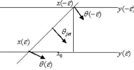
Here, we use value xjet as the consequence of truncating domain around
ξ= 0, and we jump from one free boundary to the other. This value is determined geometrically, as illustrated in Figure 2.
Figure 2: Geometry ofxjet
From the separation pointA, we can calculatex(ǫ) andy(ǫ); and from point
Finally, the distance of the vertical wall to the vertical axis is
l=x(ξb).
4. NUMERICAL CALCULATIONS
The analytical solution θ(ξ) has been derived in the previous section. This function is then used to determine the coordinates (x, y) of the free boundaries of the jet. We calculate some points (x, y) numerically, since the integrations (15) and (16) are not simple. While they are obtained, the jet is performed as plot of them with a uniquel andθjetfor each value ξb.
4.1. Numerical Procedure
The numerical procedure is begun by discretizing (ξb,−ǫ)S(ǫ,1), where the
first interval is divided intoM subinterval and the second one intoN subinterval. Each subinterval is defined by taking the same length of subinterval in φ, to get better accuracy. If we define φb = −π1log(|ξb|) and φǫ = −1πlog(ǫ), the set of
to approximate the integration in (15) and (16) by trapezoidal rules, to obtain the coordinates of the free surface of the jet.
In applying the procedure we evaluate the values ofxandy, for the bottom boundary of the jet, using
xj=xj+1+
the coordinates of the separation point on the bottom wall, that are chosen as the center coordinates.
We then continue to evaluate the coordinates of the other free surface. The value of y is computed similar to (17), but it is started from the separation point on the vertical wall, i.e.
yj =yj−1−
upper free surface, is determined by
xjet=
tan(θjet+π/2)
.
For the other values of xj, j =M −1, M−2,· · ·,0, we evaluate using (17). The
last value ofxrepresents the distance of of the vertical wall to the vertical axisl.
4.2. Results
Most of our calculations uses M = 100 grids andǫ = 0.01. These numbers are able to give four-figure accuracy forl. This accuracy is observed following the method in Wiryanto & Tuck [6] for some variousM.
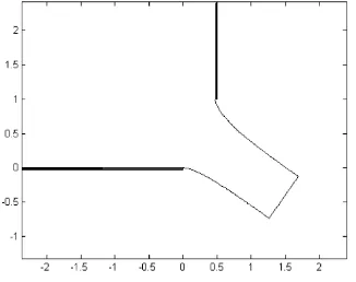
Figure 3: Plot of a jet emerging from a slit withl= 0.4687
As the result, we show in Figure 1(a) a typical jet emerging from a slit for the vertical wall being on the left vertical axis,l=−0.3636 (equivalent withξb=−10),
producingθjet=−17.55 degree. When we increase l, the jet emerges with smaller
θjet. This is shown in Figure 3 forl = 0.4687 (equivalent withξb = −2) to give
a comparison to the previous calculation. We obtain that the jet emerges with smaller asymptotic angleθjet=−35.26 degree.
For some various ξb we calculate l and θjet, and we show plot of them in
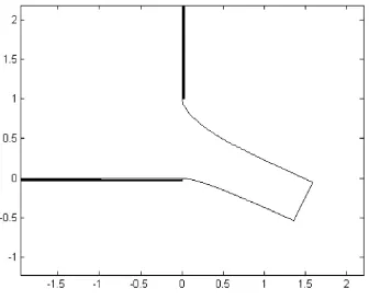
Figure 4. The value ofl= 0, the vertical wall is on the vertical axis, is obtained for ξb=−4.541 and producingθjet=−25.19. Plot of the jet is performed in Figure 5.
Figure 5: Plot of jet emerging from a slit withl= 0
5. CONCLUSION
We have solved the extreme case of a flow producing a jet emerging from a slit, in which the effect of gravity is assumed to be negligible. The analytical solution is obtained in term of the tangential of the curve boundary of the jet, and the profile of the jet is performed by plotting some points calculated from an integration involving that analytical solution. We found that the jet emerges downward asymptotically to a uniform stream with angle θjet, depending on the
position of the vertical wall to the vertical axisl.
1. F. Dias and E.O. Tuck, “Weir flows and waterfalls”, J. Fluid Mech. 320(1991),
525-539.
2. K.H.M. Goh,Numerical solution of quadratically nonlinear boundary value problems using integral equation techniques, with applications to nozzle and wall flows, Ph.D. thesis, Department of Applied Mathematics, The University of Adelaide, 1986. 3. E.O. Tuck and J.-M. Vanden-Broeck, “Ploughing flows”,Euro. J. Applied Math.,
9(1998), 463-483.
4. L.H. Wiryanto, Some nonlinear shallow-water flows, Ph.D. thesis, Department of Applied Mathematics, The University of Adelaide, 1998.
5. L.H. Wiryanto, “Zero gravity of free-surface flow over a weir”,Proc. ITB31(1999), 1-4.
6. L.H. Wiryanto and E.O. Tuck, “A back-turning jet formed by a uniform shallow
stream hitting a vertical wall”,Proc. Int. Conf. on Dif. Eqs.: ICDE’96, E. Soewono and E. van Groesen (eds.), Kluwer Academic Press, 1997.
L.H. Wiryanto: Department of Mathematics, Jalan Ganesha 10, Institut Teknologi