Full Terms & Conditions of access and use can be found at
http://www.tandfonline.com/action/journalInformation?journalCode=cbie20
Download by: [Universitas Maritim Raja Ali Haji] Date: 19 January 2016, At: 19:58
Bulletin of Indonesian Economic Studies
ISSN: 0007-4918 (Print) 1472-7234 (Online) Journal homepage: http://www.tandfonline.com/loi/cbie20
Fiscal sustainability and solvency: theory and
recent experience in Indonesia
Stephen V. Marks
To cite this article: Stephen V. Marks (2004) Fiscal sustainability and solvency: theory and recent experience in Indonesia, Bulletin of Indonesian Economic Studies, 40:2, 227-242, DOI: 10.1080/0007491042000205295
To link to this article: http://dx.doi.org/10.1080/0007491042000205295
Published online: 19 Oct 2010.
Submit your article to this journal
Article views: 110
View related articles
ISSN 0007-4918 print/ISSN 1472-7234 online/04/020227-16 © 2004 Indonesia Project ANU DOI: 10.1080/0007491042000205295
FISCAL SUSTAINABILITY AND SOLVENCY:
THEORY AND RECENT EXPERIENCE IN INDONESIA
Stephen V. Marks* Pomona College, Claremont CA
A major challenge for Indonesian economic policy makers is to avoid the recur-rence of conditions that could trigger a new economic crisis. One of the important dimensions of this challenge will be to conduct fiscal policy in a way that is sustain-able, given the level of interest rates and the rate of growth of the economy. This paper synthesises various approaches to the measurement of fiscal sustainability that have appeared in the economic literature, relates these measures to the funda-mental concept of fiscal solvency, and applies the framework to Indonesia over the period 1991–2003. The domestic and foreign debt positions of the central govern-ment are treated separately, to capture the influence of exchange rate changes on the relative costs of domestic and foreign borrowing. The empirical analysis indi-cates that Indonesia has met the fiscal sustainability criterion in recent years, except when the rupiah has depreciated heavily.
As Indonesia moves forward from the economic crisis of 1997–98, and away from the tutelage of the International Monetary Fund (IMF), it is imperative that the central government manage the economy so as to maintain confidence and pro-mote growth. One of the essential aspects of this task is the appropriate manage-ment of fiscal policy. Fiscal managemanage-ment will not be easy in the years ahead, par-ticularly given the complexities of fiscal decentralisation and the weight of the obligations the government now bears as a result of the banking crisis. For confi-dence to be maintained, and future crises to be averted, it is necessary that fiscal policy be in a fundamental sense sustainable. Although fiscal sustainability indi-cators such as the budget deficit or debt relative to GDP are readily available, a variety of more sophisticated indicators of the overall fiscal position of the cen-tral government have been proposed in recent years. Such indicators take into account that a given ratio of debt to GDP will be less problematic the higher the rate of real GDP growth relative to real interest rates.
The analysis presented in this paper looks at the fiscal position of the central government only. Thus, the appropriate debt variable is gross central government debt issued to domestic and foreign lenders. The central bank is one of these lenders, and seigniorage revenues associated with central bank lending to the central government are thus accounted for.1Fiscal positions of provincial or local governments are excluded from the analysis, owing primarily to problems of data availability and consistency. In defence of this simplification, Indonesian provinces and local governments so far have not been allowed to issue debt of their own.
The framework developed here is a hybrid of those of Blanchard (1990) and Buiter (1995). Blanchard provided a basic treatment of the approach, but Buiter made valuable contributions through his separate treatment of domestic and for-eign debt, and through use of a notation based on discrete time intervals, which provides a clearer basis for empirical work than does continuous time. On the other hand, Buiter includes variables related to the government capital stock that are not easily observable, and in this respect I have adopted a simpler approach, more like that of Blanchard, in order to keep the empirical analysis tractable.
A related econometric literature posits that if real deficits or debt are stationary time series or, alternatively, if government revenues and expenditures are co-integrated, then there is evidence of fiscal sustainability.2 These econometric analyses are retrospective, and have allowed for endogenous breaks in the fiscal regime. However, for the case of Indonesia, the simplicity of the approach pre-sented in this paper has two main advantages. First, it allows for close examina-tion of year-by-year developments in the sustainability of fiscal policy, with some diagnostic capabilities that are useful for policy makers. Second, it does not require a lengthy time series of consistent data.
The next five sections of the paper lay out the theoretical issues. The first sec-tion examines the fundamental solvency constraint that applies to a government over the long run, while the next considers the short-run dynamics of the govern-ment budget. The third section defines the concept of fiscal sustainability in gen-eral terms, and discusses the simplest indicator of fiscal sustainability. The fourth section examines the relationship between this simple fiscal sustainability indica-tor and the fundamental solvency constraint for the government, while the fifth discusses the strengths and weaknesses of the indicator. The final section presents an empirical analysis of recent experience in Indonesia based on application of the indicator.
LONG-RUN FISCAL SOLVENCY
We first examine the fundamental intertemporal budget constraint under which a government operates over time; Chalk and Hemming (2000) call this the pres-ent value budget constraint. Consider in particular the relationship between gov-ernment debt in one period and the next, and for simplicity suppose for the moment that all debt is issued in the domestic currency. The relationship can then be written as:
(1)
where Btis debt at the end of period t, itis the nominal interest rate in period t, and Stis the primary surplus in period t. The primary surplus is equal to the over-all government surplus, but with interest payments excluded. More detailed expressions for Btand Stwill be provided later.
Relationship (1) can be solved forward to a terminal period Tfrom an initial period 0 to obtain an intertemporal budget constraint for the government. Suppose for simplicity that the interest rate iis constant over time. Then we get:
Bt ≡(1+i Bt) t−1−St
228 Stephen V. Marks
(2)
Now, divide by (1 + i)Tand rearrange to solve for B
0, then take the limit of the resulting expression as the terminal time period Tapproaches infinity (∞):
(3)
The term in square brackets is the present value of the terminal debt stock. A nec-essary condition for fiscal sustainability is that this be equal to zero: in other words, the debt must be growing more slowly than the rate of interest. If the term in square brackets were positive, then the government would be rolling over its debt into the indefinite future, as in a kind of Ponzi game.3With the term in square brackets equal to zero, the intertemporal budget constraint is simply:
(4)
The intuition is that the present value of future surpluses must exceed the pres-ent value of future deficits by an amount exactly equal to the initial level of debt, so that the debt is paid off in the long run. It will be shown later that an easy-to-compute measure of fiscal sustainability bears a close relationship to this sol-vency condition.
CENTRAL GOVERNMENT DEBT DYNAMICS
We now look more closely at government finances, with the various components of the budget specified in detail, and allowing for government debt to be held domestically and internationally. The approach draws heavily on Buiter (1995), but simplifies his analysis in a number of ways that make it easier to apply.
The single period government budget constraint in period tis as follows:
(5) The left side shows the deficit, the right side how it is financed. In particular:
Ct is the nominal value of government consumption spending in period t; At is the nominal value of government capital formation in period t; Tt is the nominal value of taxes net of transfers and subsidies in period t; Et is the nominal exchange rate, defined as the number of rupiah per dollar,
in period t;
is the dollar value of foreign aid in period t;
Ft is the nominal value of gross cash flow from the public sector capital stock in period t;
Vt is the nominal value of privatisation revenues in period t;
it is the nominal interest rate on rupiah-denominated central government debt in period t;
is the nominal face value of the gross stock of rupiah-denominated debt of the central government at the end of period t;
is the nominal interest rate on foreign currency-denominated central gov-ernment debt in period t; and
is the nominal dollar value of the gross stock of foreign currency-denominated debt of the central government at the end of period t.
The right side of equation (5) indicates that the central government finances a deficit in period tby issuing additional debt denominated in either rupiah or for-eign currency. The central government surplus in period tis the negative of the left side of equation (5). The primary surplus of the central government in period t, denoted by St, is equal to this overall surplus, except that interest payments are omitted:
(6)
The nominal rupiah value of the total gross stock of central government debt at the end of period tis given by Bt:
(7)
Equation (5) can now be rearranged, and simplified based on equations (6) and (7), to show the evolution of the debt over time:
(8)
is the rate of appreciation of the dollar against the rupiah in period t.
Divide both sides of equation (8) by nominal GDP, equal to P
tYt, so as to
express all terms as ratios to GDP in period t:
(9)
Rewrite (10), using lowercase letters to indicate the original variable relative to GDP:
(11)
where:
is total central government debt at the end of period t, measured in rupiah, as a fraction of GDP in period t;
is central government debt denominated in rupiah at the end of period t, as a fraction of GDP in period t;
is central government debt denominated in foreign currency at the end of period t, as a fraction of GDP in period t; and
is the primary central government surplus as a fraction of GDP in period t.
Finally, using the definition of the real interest rate rtin period t:
(12)
and using the fact that , equation (11) can be rewritten as:
(13)
In the expression for btin equation (13), the first term applies the domestic real interest rate to the entire domestic and foreign debt. The second term shows the excess cost of borrowing by issuing foreign currency-denominated debt rather than rupiah-denominated debt, which could be positive or negative, multiplied by the stock of foreign debt relative to GDP. Buiter states that the term in square brackets in equation (13) corrects for deviations from uncovered interest parity,4 but this is not exactly correct in general.5
To simplify the notation, Buiter defines the augmented primary surplus to GDP ratio:
(14)
This augmented ratio equals the primary surplus to GDP ratio, adjusted for the excess cost of borrowing internationally rather than domestically, which is then multiplied by the ratio of foreign debt to GDP. The process that describes the evo-lution of the central government debt can then be written simply as follows:
(15)
FISCAL SUSTAINABILITY INDICATORS
Fiscal sustainability is the capacity to maintain the current fiscal stance without needing to make adjustments in tax or expenditure policies in order to assure sol-vency as defined by the present value budget constraint (equation 4).
If we seek an indicator of fiscal sustainability, need we perhaps look no further than the ratio of the public deficit to GDP, or the ratio of the stock of public debt to GDP? An increase in either of these ratios would seem to indicate a more prob-lematic fiscal position for the government, insofar as GDP reflects the potential for tax revenues to be collected. Of course, this potential will vary from country to country, and can vary within a given country over time, subject to its level of institutional development and the structure of its economy.6Thus, comparison and interpretation of such ratios must be undertaken with caution.
Suppose that our goal is simply to predict the ratio of debt to GDP in the next period. Equation (15) shows that a lower primary surplus will not necessarily be associated with a higher subsequent debt to GDP ratio (bt), since it could be off-set by a lower real interest rate (rt), a higher real growth rate (gt), or a lower ini-tial debt to GDP ratio (bt–1). Similarly, a higher initial debt to GDP ratio will not necessarily lead to a higher subsequent debt to GDP ratio, since it could be offset by a lower real interest rate, a higher real growth rate, or a larger primary surplus.
We need a more sophisticated indicator of fiscal sustainability, then, one that takes into account the interrelationships among these variables. A variety of such indicators have been discussed in the literature. This paper will focus on the sim-plest measure that Blanchard, Buiter and others have proposed. The goal in par-ticular is to find the augmented primary surplus to GDP ratio that, if maintained over time, will hold the debt to GDP ratio constant at its initial level. It will be assumed for simplicity that the real interest rate and the real rate of growth will remain constant over time, at rates rand g, respectively.
Let be the augmented primary surplus to GDP ratio that will be maintained over time, and let b0be the debt to GDP ratio in period 0. For the debt to GDP ratio to remain constant over time, its value in period 1, b1, will have to equal b0, as will the debt to GDP ratio in all later time periods. Using equation (15), we thus require:
(16)
which can be solved for to yield the required augmented primary surplus:
(17)
The ‘one-period primary gap’ indicator of fiscal sustainability proposed by Blanchard and Buiter is then equal to the difference between the required aug-mented primary surplus given by equation (17) and the actual augaug-mented pri-mary surplus. If this gap is positive, it indicates that the required pripri-mary surplus is higher than the actual primary surplus, implying that fiscal adjustment will have to occur at some time in the future if the ratio of debt to GDP is not to increase. If it is negative, then the debt to GDP ratio will shrink over time under the assumption that the primary surplus to GDP ratio and the other relevant vari-ables remain constant.
The one-period primary gap can be calculated for a succession of time periods, to determine how the posture of fiscal policy is changing over time. These one-period calculations are naïve in that the relevant economic and fiscal variables are assumed to remain constant over time, but are easy to perform because econo-metric forecasts of future paths of economic and fiscal variables are not required. There are multi-period versions of the primary gap indicator that relax the assumption that the relevant variables (notably the real interest rate and the real growth rate) will remain constant over time, and instead use forecasts of these variables for future periods (see Buiter 1995 for details). Such approaches would be most useful if policies or conditions are expected to change significantly in the future.
THE PRIMARY GAP INDICATOR AND FISCAL SOLVENCY
It is important to understand clearly the relationship between the primary gap indicator and fiscal solvency. First, both sides of the solvency condition, equation (4), can be restated in terms of variables that are defined relative to nominal GDP. Following the approach in earlier sections, suppose for simplicity that the growth rate of real GDP, the real interest rate and the inflation rate will be constant into the indefinite future, at rates g, rand π, respectively. Next, define:
and
In addition, note that:
and
Then, using the definition of real interest rates in equation (12), equation (4) can be rewritten as:
(18)
Now let s* represent a constant primary surplus to GDP ratio that will be main-tained over time. Under the assumption that r> g,7 equation (18) can then be solved for s*:
(19)
Notice that the expression for s* in equation (19) is identical to the expression for in (17).8This equivalence provides an alternative interpretation of the one-period required primary surplus, under the condition that r> g: it is the primary surplus to GDP ratio that, if held constant over time, given that the real interest rate and the growth rate also remain constant into the indefinite future, would allow the government to remain solvent.9
Recall for comparison the original rationale for the required primary surplus: it was the primary surplus to GDP ratio that, if held constant over time, would
˜
234
Stephen V
. Marks
TABLE 1 Data and Calculations for the One-period Primary Gap Indicator of Fiscal Sustainability, 1991–2003 (Rp trillion, unless indicated otherwise)
1990 1991 1992 1993 1994 1995 1996 1997 1998 1999 2000 2001 2002 2003
Consolidated central government stock variables
Foreign debt, end of period 85.9 87.4 105.5 118.8 138.8 136.8 127.3 236.7 467.3 464.1 614.6 627.0 586.8 565.6
Ratio to GDP (%) 40.7 35.0 37.4 36.0 36.3 30.1 23.9 37.7 48.9 42.2 48.6 43.3 36.4 31.7
Domestic debt, end of period 3.6 4.2 5.4 4.9 0.9 3.2 0.1 4.1 100.0 496.6 653.9 659.0 650.7 623.9
Ratio to GDP (%) 1.7 1.7 1.9 1.5 0.2 0.7 0.0 0.7 10.5 45.2 51.7 45.5 40.4 34.9
Total debt, end of period 89.5 91.6 111.0 123.7 139.8 140.0 127.4 240.8 567.3 960.7 1,268.5 1,286.0 1,237.5 1,189.5
Ratio to GDP (%) 42.4 36.6 39.3 37.5 36.6 30.8 23.9 38.4 59.4 87.4 100.3 88.7 76.8 66.6
Consolidated central government flow variables
Total revenue and grants 39.6 42.4 50.6 56.3 69.5 80.4 90.3 113.9 157.4 198.7 273.8 301.1 300.1 336.2
Total expenditure 38.7 41.3 52.2 55.0 61.9 66.7 78.0 112.9 174.1 223.5 295.3 341.6 327.1 370.6
Interest payments 5.0 4.6 5.4 6.3 7.6 7.1 6.4 10.8 31.3 42.9 66.8 87.1 89.9 82.0
Primary surplus 5.9 5.7 3.8 7.7 15.2 20.8 18.8 11.8 14.6 18.1 45.2 46.7 62.9 47.6
Actual primary surplus to GDP ratio (%) 2.8 2.3 1.4 2.3 4.0 4.6 3.5 1.9 1.5 1.6 3.6 3.2 3.9 2.7
Correction factor for interest differentials –0.03 –0.02 0.00 0.00 –0.02 –0.04 0.66 0.01 –0.29 0.23 –0.05 –0.24 –0.11
Augmented primary surplus to GDP ratio (%) 3.5 2.1 2.4 3.8 5.4 4.8 –13.9 1.2 15.7 –6.3 5.6 14.5 6.8
Nominal domestic interest rate (%) 14.0 14.9 12.0 8.7 9.7 13.6 14.0 27.8 80.6 26.2 15.4 19.5 16.6 11.7
Real domestic interest rate (%) 3.7 5.5 –0.9 1.8 3.4 4.9 13.5 3.1 10.6 5.3 7.9 8.8 4.8
Public and guaranteed foreign debt ($ billion) 48.0 51.9 53.7 57.2 63.9 65.3 60.0 55.9 67.3 73.4 69.4 68.4 65.6 69.8
Interest payments on this debt ($ billion) 2.8 2.9 3.0 3.2 3.2 3.8 3.6 3.2 3.0 3.8 3.8 3.6 2.7 3.1
Imputed interest rate on public foreign debt (%) 6.1 5.8 6.0 5.7 5.9 5.5 5.4 5.3 5.6 5.1 5.2 4.0 4.8
Exchange rate, end of period (Rp/$) 1,901 1,992 2,062 2,110 2,200 2,308 2,383 4,650 8,025 7,085 9,595 10,400 8,940 8,465
Rate of appreciation of dollar against rupiah (%) 4.8 3.5 2.3 4.3 4.9 3.2 95.1 72.6 –11.7 35.4 8.4 –14.0 –5.3
Gross domestic product
Nominal GDP 210.9 250.0 282.4 329.8 382.2 454.5 532.6 627.7 955.8 1,099.7 1,264.9 1,449.4 1,610.6 1,786.7
Real GDP (1995 = 100) 70.9 75.8 80.7 85.9 92.4 100.0 107.8 112.9 98.1 98.8 103.7 107.3 111.2 115.8
Real GDP growth (%) 7.0 6.5 6.5 7.5 8.2 7.8 4.7 –13.1 0.8 4.9 3.4 3.7 4.1
GDP deflator (1995 = 100) 65.5 72.6 77.0 84.4 91.0 100.0 108.7 122.3 214.4 244.8 268.4 297.3 318.6 339.4
GDP inflation rate (%) 10.8 6.1 9.6 7.8 9.9 8.7 12.6 75.3 14.2 9.6 10.8 7.2 6.5
Required one-period primary surplus to GDP ratio (%) –1.3 –0.3 –2.7 –2.0 –1.6 –0.8 2.0 7.1 5.8 0.3 4.3 4.4 0.5
One-period primary gap (%) –4.8 –2.5 –5.1 –5.8 –7.0 –5.6 15.9 5.9 –9.9 6.6 –1.3 –10.1 –6.2
hold the debt to GDP ratio constant, under the assumption that other factors like inflation, real interest rates and the real economic growth rate remained constant.
STRENGTHS AND LIMITATIONS OF THE PRIMARY GAP INDICATOR
The above analysis implies that the required primary surplus concept, and thus the primary gap fiscal sustainability indicators that are based on it, are more gen-eral than initially might have been supposed.
However, it must be acknowledged that the constancy of the primary surplus over time relative to GDP is a strong and arbitrary restriction. Chalk and Hemming (2000) note that meeting the present value budget constraint (PVBC), the fundamental solvency constraint given by equation (4), in reality does not even require that the debt to GDP ratio be bounded, much less that it be constant. Thus, a government that meets the fiscal sustainability condition given by equa-tion (17) will certainly satisfy the PVBC, but it is not necessary to satisfy equaequa-tion (17) in order to satisfy the PVBC. Buiter recognises this limitation of his frame-work, and in its defence notes that in practice debt to GDP ratios will have to be bounded if policy is to remain credible. Indeed, Chalk and Hemming conclude that indicators like the one-period primary gap can constitute a prudent approach to testing for fiscal sustainability in many cases in which a government has high debt and high primary deficits.
One does not want to rely on fiscal sustainability indicators to the exclusion of other considerations, however. For example, sustainability per se may be less important than economic recovery in the short run, if the economy has suffered a negative shock. Therefore, to support the long-run health of the economy, and thus the long-run viability of government finances, increased ratios of deficits or debt to GDP may sometimes be optimal, particularly if the economy cannot read-ily find its own way back to a high-employment, high-output equilibrium.
As is well known, some of this change in fiscal policy will occur automatically. For example, tax revenues typically go down during a recession. This reduction in taxes then partly cushions the economy against the recession. If the budget is not tightened to offset the lower tax revenues, it will shift toward deficit, and the public debt could grow as well. Since real GDP is by definition shrinking during a recession, the deficit to GDP ratio will increase, and the debt to GDP ratio could increase as well. Over the long run this could be better for the economy and ernment finances than if these ratios remained constant or went down. The gov-ernment may also wish to consider discretionary fiscal policies in order to pro-vide additional stimulus to economic activity. A risk is that excessive stimulus could undermine confidence and lead to inflation, depreciation and markedly higher interest rates. The question then arises as to the optimal level of the gov-ernment debt over time. Such an inquiry extends beyond the scope of this paper, but see Elmendorf and Mankiw (1999) for a survey of the issues.
EMPIRICAL ANALYSIS APPLIED TO INDONESIA
The one-period primary gap indicator can be readily calculated over a recent span of years for Indonesia. Table 1 shows the relevant data and calculations for each of the fiscal years from 1991 to 2003.10
The foreign and domestic debt data are from the International Financial Statistics (IFS) of the IMF through 1996 and 1997, respectively, and from World Bank (2003) for more recent years through 2002.11The figures in table 1 include debt incurred by the central government only, and do not include loans from the IMF, which have served to provide additional foreign exchange reserves to the central bank (as distinct from budgetary support). Consolidated central government flow vari-ables are from the Government Finance Statistics Yearbook(GFS) of the IMF through 1999, and from the Ministry of Finance for 2000–03.12Total revenues include cash flows from government capital, and in principle could include privatisation rev-enues as well. Expenditures include both current and capital account items.13
The primary surplus is derived from the above figures. The correction factor for interest differentials is the term in square brackets from the definition of the augmented primary surplus to GDP ratio in equation (14), which uses data described below.
The question of which interest rate is most representative for domestic debt is difficult, since the nature of the government debt instruments has changed over time and the data are incomplete. Before the economic crisis, domestic debt of the central government was negligible and was not publicly traded. However, gov-ernment obligations exploded owing to the collapse of the banking system. The government issued non-tradable long-term debt to Bank Indonesia in 1998–99 to compensate it for its last resort lending to the banks. This was in two forms: the vast majority guaranteed a return equal to the rate of inflation of the consumer price index (CPI) plus 3%, while a much smaller amount paid a variable return equal to the three-month SBI (Sertifikat Bank Indonesia, Bank Indonesia Certificate) rate.
By 1999 the government began to issue tradable variable and fixed rate long-term bonds of various maturities, as well as much smaller amounts of non-publicly-traded hedge bonds.14 Initially these bonds were injected directly into banks’ balance sheets, under the bank recapitalisation program. More recently, they have been offered to the public at market-determined prices; data on trans-action prices and the associated yields for new bond issues have been available since July 2001.15There have been buy-backs of some of the debt along the way. By the end of May 2004, 55.4% of the domestic debt outstanding was in the form of variable rate bonds, 42.2% was in fixed rate bonds, and 2.4% in hedge bonds. The effective yields on the variable and fixed rate bonds at the time of issue have been very similar.16
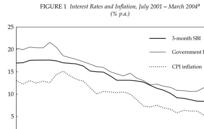
Figure 1 shows the weighted average yield on newly issued long-term fixed and variable rate government bonds, the three-month SBI rate, and the rate of CPI inflation over the previous 12 months, for the period during which the market-determined bond yield data have been publicly available.17Since January 2002, as inflation has diminished and stability has returned, the spreads on govern-ment bond yields relative to both the three-month SBI rate and CPI inflation have mostly narrowed.18
For the present analysis I represent the domestic interest rate paid by the gov-ernment as follows. For 1990 through 1997 it is the short-term money market rate from IFS. For 1998 it is the rate of CPI inflation plus 3%, to represent the yield on the guaranteed debt issued to Bank Indonesia at the time. For 1999 and afterward it is the estimated or actual weighted-average yield on newly issued long-term
236 Stephen V. Marks
government bonds.19,20The real domestic interest rate is calculated on the basis of actual inflation of the GDP deflator and the nominal domestic interest rate.
The foreign interest rate is imputed on the basis of the stock of long-term pub-lic and pubpub-licly guaranteed foreign debt at the end of the previous year and inter-est payments on that debt during the given year, as reported in Global Development Finance: Country Tables (GDF), published by the World Bank.21 (In effect, it is assumed that all transactions occur on the last day of each year.) The imputed interest rates appear to be relatively low; this may be because a higher percentage of this debt has been on concessional terms for Indonesia than for all developing countries as a group (41% versus 27% at the end of 2001, for exam-ple). However, the concessional agreement between Indonesia and the Paris Club of creditor governments ended in December 2003, and Indonesia will incur higher costs in the future as it relies more on foreign commercial credit.22
The exchange rate data are end-of-year figures from IFS. The gross domestic product data are from IFSthrough 2001, and from the Central Statistics Agency (BPS) for 2002–03.23Table 1 reveals that the real rate of interest has exceeded the GDP growth rate since 1997. Since calculation of the one-period primary gap indicator presupposes that these variables will remain constant over time, the dis-cussion related to equation (19) implies that the primary gap indicator can be related directly to the fiscal solvency constraint. Before 1997 the real interest rate was less than the real rate of growth. Nevertheless, based on the definition of the primary gap indicator, even for these years we can say that the debt to GDP ratio would have remained constant over time if the primary gap indicator had been
FIGURE 1 Interest Rates and Inflation, July 2001 – March 2004a (% p.a.)
a The rate for government bonds is the weighted average yield on newly issued long-term fixed and variable rate bonds.
Sources: See note 17.
Jul-20010 Jan-2002 Jul-2002 Jan-2003 Jul-2003 Jan-2004
5 10 15 20 25
3-month SBI
Government bonds CPI inflationequal to zero and if the growth rate, inflation rate, interest rate and ratio of the primary surplus to GDP had remained constant.
The calculations of the one-period primary gap for Indonesia show the gap to be comfortably negative for much of the period from 1991 to 2003. For example, in 1996 the gap was –5.6% of GDP. The negativity of the gap indicated that, if the augmented primary surplus, the real GDP growth rate and the real interest rate were continued into the indefinite future, the ratio of public debt to GDP would diminish over time. Given the uncertainty about domestic and foreign nominal interest rates, I performed some sensitivity analysis by setting these to ±20% of the figures given in table 1 throughout the period, and found that the results var-ied in reasonable ways and not by very much. For example, if the domestic inter-est rate had been 20% higher in 2003 (14.0% rather than 11.7%), the one-period primary gap would have been –5.4% of GDP rather than –6.6%.
The only three years that exhibit fiscal sustainability problems based on the one-period primary gap indicator are 1997, 1998 and 2000. The first two years marked the onset of the economic crisis. The third witnessed deteriorating eco-nomic conditions due in part to a loss of confidence in the government of Abdurrahman Wahid. Closer examination of the data for these three years is instructive:
• Real GDP growth was negative only in 1998. It was higher in 1997 and 2000 than it has been in any other year since 1996. In none of these other years did the primary gap indicate any significant problem.
• Similarly, the GDP inflation rate was very high in 1998, but in 1997 and 2000 it was close to or lower than in 1999 or 2001. In 2002 and 2003, the inflation rate slowed relative to earlier years.
• Domestic real interest rates were relatively high in 1997 and 1999, but consid-erably lower in 1998 and 2000. Foreign interest rates were relatively stable throughout the entire period.
• The central government primary surplus was lower by about 2% of GDP dur-ing and after the economic crisis, from 1997 to 1999, than it had been earlier, but since then has returned to its recent historical range.
• There were enormous increases in both the foreign and the domestic debt of the central government during and after the economic crisis. Foreign debt peaked relative to GDP in 1998, while domestic and total debt peaked relative to GDP in 2000.
These debt increases were a crucial part of the fiscal story during this period, and were due mainly to the bank bailouts undertaken by the government. In con-sultation with the IMF, the government included in the budget only the subse-quent interest costs of these bailouts, not the initial capital costs. McLeod (2004) notes that if the initial outlays had been included as well, this would have pro-vided a truer picture of the enormity of the burden. In this case, the primary sur-pluses recorded during these years would have been considerably larger and the fiscal sustainability indicators would have painted a bleaker picture, albeit only as long as new capital costs were being incurred.
However, given the approach used to account for the bank bailouts, the factor that seems most decisive in the measured year-to-year changes in fiscal
sustain-238 Stephen V. Marks
ability in the recent past has been the behaviour of the exchange rate. In each of the three years for which Indonesia had positive one-period primary gap meas-urements—1997, 1998 and 2000—the rupiah depreciated sharply against the dol-lar. By 2000, even though total debt to GDP was peaking, depreciation of the rupiah was less than it had been in 1997 and 1998, and the primary gap indicator was much lower than it had been in 1997 and not much higher than in 1998.
The influence of the exchange rate is via the rupiah value of foreign currency-denominated debt and grants, and through the correction factor for the interest differential between foreign and domestic borrowing. Note, in particular, the con-siderable difference between the actual and augmented primary surplus to GDP ratios during most of the years since 1997. Even with a relatively stable primary surplus to GDP ratio, the augmented primary surplus to GDP ratio was highly volatile over this period. The three years in which the augmented primary sur-plus ratio turned sharply downward relative to the actual primary sursur-plus ratio were the years in which the correction for interest differentials was positive and the rupiah was losing value.
This framework shows, then, the importance of the exchange rate for fiscal conditions within Indonesia. It also shows that the one-period primary gap indi-cator of fiscal sustainability can vary substantially from year to year, even with-out major changes in underlying economic conditions or indebtedness. These observations lead to two practical conclusions. First, it is important to understand the underlying causes of changes in the primary gap as a fiscal sustainability indicator. Such understanding is useful in order to diagnose the problem, assess its severity and, if necessary, prescribe a remedy in terms of policy adjustment. Second, only if the primary gap indicator shows a sustained deterioration and positive values over a prolonged period should there be serious concern about fiscal sustainability. Temporary deterioration of the indicator can be reversed if the credibility of policy can be maintained or restored.
NOTES
* The author completed most of the work on this paper while an economist in Jakarta with the Partnership for Economic Growth, a collaborative project of the US Agency for International Development (USAID) and the Republic of Indonesia. The views in this paper are those of the author alone, and not necessarily those of USAID or the Indonesian government. The author thanks Wismana Adi Suryabrata, William Wallace, Slavi Slavov, Michael Kuehlwein and two anonymous referees for helpful dis-cussion and comments.
1 The seigniorage per se is due to the expansion of the monetary base (equal to bank reserves plus currency in circulation) associated with this lending. These liabilities of the central bank do not bear interest and thus amount to an interest-free loan to the central bank.
2 Hamilton and Flavin (1986) was a seminal work in the field. Bravo and Silvestre (2002) and Martin (2000) are recent contributions, and survey previous studies.
3 O’Connell and Zeldes (1988) provide a comprehensive treatment of the theory. 4 Uncovered interest parity holds if the rates of return on domestic currency
interest-bearing assets and on similar foreign currency interest-interest-bearing assets are equal, after adjustment for expected exchange rate changes. That the investment in the foreign cur-rency asset is ‘uncovered’ means that the investor is exposed to the risk that the foreign
currency will unexpectedly change in value against the domestic currency. If forward markets in foreign currency are available, investors instead may be able to cover their positions so as to avoid currency risk.
5 If the numerator of this term contained the expected rate of appreciation of foreign cur-rency rather than the actual rate of appreciation, and if the numerator were equal to zero, then uncovered interest parity would hold. The actual and expected rates of appreciation of foreign currency would be equal in general only if individuals had per-fect foresight.
6 Demographics could be one aspect of this structure. For example, the number of eld-erly in many industrial countries will grow substantially within several decades, cre-ating a major burden on the fiscal system. Indonesia does not face a demographic prob-lem of this sort, and does not have general income supports for the elderly.
7 This assumption has been met in Indonesia since 1997, but was not met prior to then, as the empirical analysis in the final section will show.
8 Recall that the required primary surplus in equation (17) corrects for differences in the cost of borrowing in domestic and in foreign currency. The s* expression in equation (19) would do so as well, were we to distinguish between domestic and foreign bor-rowing in its derivation.
9 The analysis is more complicated, but essentially unchanged, if the interest rate or the growth rate varies over time.
10 Some of the data are needed for 1990 as well, and these are also shown in the table. 11 The external debt figures in the source include debt owed to the IMF, which I have
removed using data from IFS. The domestic debt figure for 1998 is from World Bank, Indonesia Office, ‘Indonesia’s Central Government Debt Outstanding’, online at lnweb18.worldbank.org/eap/eap.nsf/Attachments/Govtdebt/. The 2003 domestic and foreign debt figures are from unpublished sources within the Indonesian govern-ment.
12 Departemen Keuangan, Nota Keuangan dan Anggaran Pendapatan dan Belanja Negara, various years, online at www.fiskal.depkeu.go.id/Utama.asp?utama=1070000. In 2000 the fiscal year was changed from 1 April – 31 March to coincide with the calendar year. I have done a rough annualisation of the central government flow variables figures for that year by multiplying the nine-month figures by 12/9.
13 Buiter (1995) takes the analysis of the consolidated central government capital account further—by relating government capital formation, privatisation, depreciation and cash flow from government capital to the stock of government capital in the current and previous period. Such an approach was not practical for Indonesia owing to data limitations, and so the primary surplus derivable directly from total revenues, total expenditures and interest payments is used.
14 Hedge bonds are rupiah-denominated bonds with the characteristics of dollar-denominated bonds, since the principal amount is indexed to the dollar. They were issued only to two of the state-owned banks.
15 These market placements have been done primarily through bond dealers, but in 2003 public auctions were initiated as well, as authorised by Law No. 24/2002 on Government Debt Instruments (Surat Utang Negara).
16 The quarterly payments from variable rate bonds are determined by applying the yield on three-month SBIs from the previous month to the face value of the bonds. SBIs are debt instruments used by Bank Indonesia for purposes of monetary control. It is much more common for central banks to trade not in their own debt but in debt of the cen-tral government. In 2005, the SBIs may begin to be replaced by Surat Utang Negara, short-term debt instruments to be issued by the government.
17 I calculated the weighted averages using data on yields to maturity for fixed and vari-able rate bond issues reported in various issues of the Quarterly Bulletin (Berita
Tri-240 Stephen V. Marks
wulan) of the Centre for Management of Indonesian Bonds (Pusat Manajemen Obligasi Indonesia) at the Ministry of Finance, online at www.dmo.or.id. SBI data are from Bank Indonesia, and the CPI data are from IFS.
18 The mutual fund crisis toward the end of 2003 described by Kenward (2004) led to a sell-off of government bonds that drove up their yields. These yields had started to set-tle down in March and April 2004, but then in May additional financial disturbances affected the government bond market; for further details see Marks (2004), the ‘Survey of Recent Developments’ in this issue.
19 I estimate bond yields for January 1999 – June 2001 as the three-month SBI rate plus the average spread over that rate from July to December 2001. As noted earlier, the fixed and variable rate bonds were initially provided directly to the banks under the recap-italistion program. These transactions were not mediated by the market, but it can be argued that it makes sense to add the later market premium over the SBI rate in order to impute a market interest rate to them. First, yields to maturity for fixed and variable rate bonds have been quite similar, as noted earlier. Second, the bonds have sold at a discount relative to face value, implying an effective interest yield for variable rate bonds above the SBI rate (see note 16).
20 A better indicator of the cost of funds to the government would be the yields on vari-able and fixed rate bonds from the secondary market, where rates are genuinely mar-ket determined. These data are given daily in newspapers, but have not been pub-lished for longer periods.
21 It would be better to include public but not publicly-guaranteed debt in the calcula-tions, but GDF,which offers the most consistent series of data back to 1990, does not report separate figures. I use these data only to impute a foreign interest rate; separate series are used for the stock of foreign public debt, as noted earlier. On the assumption that interest rates on publicly-guaranteed debt are close to those on public debt, any bias in the imputed interest rate should be small. Because GDFdata were not available for 2002 and 2003, it was necessary to use foreign public debt data from the World Bank and foreign interest payments reported in the budget by the Ministry of Finance for these years, from the sources cited in footnotes 11 and 12.
22 In March 2004, the government issued $1 billion worth of 10-year foreign debt with a yield of 6.85%, and it was eagerly welcomed by foreign creditors.
23 BPS is online at www.bps.go.id/index.shtml; the figures for 2002 come from statistical tables and those for 2003 from a press release.
REFERENCES
Blanchard, Olivier J. (1990), ‘Suggestions for a New Set of Fiscal Indicators’, Organisation for Economic Co-operation and Development Working Paper No. 79 (April), OECD, Paris, www.oecd.org/dataoecd/16/41/2002735.pdf.
Bravo, Ana Bela Santos, and Antonio Luis Silvestre (2002), ‘Intertemporal Sustainability of Fiscal Policies: Some Tests for European Countries’, European Journal of Political Economy
18 (September): 517–28.
Buiter, Willem H. (1995), Measuring Fiscal Sustainability, Cambridge University, August (mimeo), www.nber.org/~wbuiter/sustain.pdf.
Chalk, Nigel, and Richard Hemming (2000), ‘Assessing Fiscal Sustainability in Theory and Practice’, IMF Working Paper WP/00/81, International Monetary Fund, Washington DC (April), www.imf.org/external/pubs/ft/wp/2000/wp0081.pdf.
Elmendorf, Douglas W., and N. Gregory Mankiw (1999), ‘Government Debt’, in John B. Taylor and Michael Woodford (eds), Handbook of Macroeconomics, Volume 1C, Elsevier Science, Amsterdam.
Hamilton, James D., and Marjorie A. Flavin (1986), ‘On the Limitations of Government
Borrowing: A Framework for Empirical Testing’, American Economic Review 76 (September): 808–19.
Kenward, Lloyd R. (2004), ‘Survey of Recent Developments’, Bulletin of Indonesian Economic Studies40 (1): 9–35.
McLeod, Ross H. (2004), ‘Dealing with Bank System Failure: Indonesia, 1997–2003’,
Bulletin of Indonesian Economic Studies40 (1): 95–116.
Marks, Stephen V. (2004), ‘Survey of Recent Developments’, Bulletin of Indonesian Economic Studies40 (2), in this issue.
Martin, Gael M. (2000), ‘US Deficit Sustainability: A New Approach Based on Multiple Endogenous Breaks’, Journal of Applied Econometrics5 (January–February): 83–105. O’Connell, Stephen A., and Stephen P. Zeldes (1988), ‘Rational Ponzi Games’, International
Economic Review29 (August): 431–50.
World Bank (2003), CGI[Consultative Group on Indonesia] Brief, Report No. 27374–IND, World Bank, Indonesia Office, December, Statistical Annex, available at: lnweb18.worldbank.org/eap/eap.nsf/Attachments/CGI-1203-CGIBrief-Annex/.
242 Stephen V. Marks