Balanced Metrics
and Noncommutative K¨
ahler Geometry
⋆Sergio LUKI ´C
Department of Physics and Astronomy, Rutgers University, Piscataway, NJ 08855-0849, USA
E-mail: [email protected]
Received March 01, 2010, in final form August 02, 2010; Published online August 27, 2010 doi:10.3842/SIGMA.2010.069
Abstract. In this paper we show how Einstein metrics are naturally described using the quantization of the algebra of functions C∞
(M) on a K¨ahler manifold M. In this setup one interprets M as the phase space itself, equipped with the Poisson brackets inherited from the K¨ahler 2-form. We compare the geometric quantization framework with several deformation quantization approaches. We find that thebalanced metrics appear naturally as a result of requiring the vacuum energy to be the constant function on the moduli space of semiclassical vacua. In the classical limit these metrics become K¨ahler–Einstein (whenM
admits such metrics). Finally, we sketch several applications of this formalism, such as explicit constructions of special Lagrangian submanifolds in compact Calabi–Yau manifolds.
Key words: balanced metrics; geometric quantization; K¨ahler–Einstein
2010 Mathematics Subject Classification: 14J32; 32Q15; 32Q20; 53C25; 53D50
1
Introduction
Noncommutative deformations of K¨ahler geometry exhibit some extraordinary features, similar to those that appear in the description ofnquantum harmonic oscillators by the noncommutative phase space Cn. Noncommutative geometry in Calabi–Yau compactifications is expected to
play a special role when the B-field is turned on [21,15], in the formulation of M(atrix) theory [3, 7, 14], and in the large N limit of probe D0-branes [13]. Also, as we show below, one can use the geometric quantization approach to noncommutative geometry to determine1 important objects in string theory compactifications, which allow the computation of the exact form of the Lagrangian in the four dimensional effective field theory [8,9,10,11].
In this paper we show how the notion ofbalanced metrics appears naturally in the framework of K¨ahler quantization/noncommutative geometry. In the geometric quantization formalism the balanced metric appears as a consequence of requiring the norm of the coherent states to be constant; these states are parameterized by the Kodaira’s embedding of the K¨ahler manifoldM into the projectivized quantum Hilbert space. In the Reshetikhin–Takhtajan approach to the deformation quantization of M [20], the balanced metric appears as a consequence of requiring the unit of the quantized algebra of functions C∞(M)[[~]] to be the constant function1:M →
1 ∈ R. Finally, we quantize the phase space with constant classical Hamiltonian on M using
the path integral formalism; here, one considers a different class of semiclassical vacuum states which are not coherent states, and uses them to define2 a generalization of the balanced metrics (which also become Einstein metrics in the classical limit).
⋆
This paper is a contribution to the Special Issue “Noncommutative Spaces and Fields”. The full collection is available athttp://www.emis.de/journals/SIGMA/noncommutative.html
1
More precisely, what one can determine are certain metrics, known as balanced metrics, which obey the equations of motion in the classical limit.
2
The organization of the paper is as follows. In Section 2 we recall some basic facts of geometric quantization [2, 12, 22], show how the balanced metrics appear naturally in this framework, and sketch how differential geometric objects, such as K¨ahler–Einstein metrics or Lagrangian submanifolds, can be described in this language. In Section 3 we summarize the work of Reshetikhin–Takhtajan, and show how the constant function is the unit element of their quantized algebra of functions if and only if the metric on M is balanced. Finally, in Section4
we consider a different set of semiclassical vacuum states in path integral quantization and use them to define generalized balanced metrics, which differ slightly from the balanced metrics in geometric quantization.
2
Geometric quantization
Classical mechanics and geometric quantization have a beautiful formulation using the language of symplectic geometry, vector bundles, and operator algebras [2, 12, 22]. In this language, symplectic manifoldsM are interpreted as phase spaces, and spaces of smooth functionsC∞(M)
as the corresponding classical observables.
K¨ahler quantization is understood far better than quantization on general symplectic mani-folds; for this reason we only consider K¨ahler manifolds (which are symplectic manifolds endowed with a compatible complex structure). (M,L⊗κ) denotes a polarized K¨ahler manifold M with a very ample hermitian line bundle3 L⊗κ, and κ∈Z
+ a positive integer. For technical reasons,
we considerM to be compact and simply connected. We work with a trivialization ofL|U →U, whereU ⊂M is an open subset; we defineK(φ,φ¯) to be the associated analytic K¨ahler poten-tial and e−κK(φ,φ¯) the hermitian metric on L⊗κ →M. If dim
CM =n and {φi}0<i≤n is a local holomorphic coordinate chart for the open subsetU ⊂M, we can write the K¨ahler metric onM and its compatible symplectic form as
iκgi¯dφi⊗dφ¯¯=κωi¯dφi∧dφ¯¯=iκ ∂ ∂φi
∂
∂φ¯¯K(φ,φ¯)dφ i
⊗dφ¯¯.
Classically, the space (C∞(M), ω) of observables has, in addition to a Lie algebra structure defined by the Poisson bracket
{f, g}P B =ωi¯(∂if∂¯¯g−∂ig∂¯¯f), f, g∈C∞(M),
the structure of a commutative algebra under pointwise multiplication, (f g)(x) =f(x)g(x) = (gf)(x).
Quantization can be understood as a non-commutative deformation of C∞(M) parameterized by ~, with commutativity recovered when~= 0. We will discuss the formalism of deformation
quantization in the next section, although generally speaking, quantization refers to an assign-ment T:f → T(f) of classical observables to operators on some Hilbert space H. When M is compact, the Hilbert space will be finite-dimensional with dimension dimH= vol~nM +O(~
1−n). The assignment T must satisfy the following requirements:
• Linearity, T(af+g) =aT(f) +T(g), ∀a∈C,f, g∈C∞(M).
• Constant map 1 is mapped to the identity operator Id,T(1) = Id. • If f is a real function,T(f) is a hermitian operator.
• In the limit~→0, the Poisson algebra is recovered [T(f), T(g)] =i~T({f, g}P B) +O(~2). 3
In other words,L⊗κ
In geometric quantization the positive line bundleL⊗κ is known as prequantum line bundle. The prequantum line bundle is endowed with a unitary connection whose curvature is the sym-plectic form κω (which is quantized, i.e., ω ∈H2(M,Z)). The prequantum Hilbert space is the
space of L2 sections
L2(L⊗κ, M) =
s∈Ω0(L⊗κ) :
Z
M
hκhs,¯siω n
n! <∞
,
where hκ is the compatible hermitian metric on L⊗κ. The Hilbert space is merely a sub-space of L2(L⊗κ, M), defined with the choice of a polarization on M. In the case of K¨ahler polarization, the split of the tangent space in holomorphic and anti-holomorphic directions, T M = T M(1,0)⊕T M(0,1), defines a Dolbeault operator on L⊗κ, ¯∂: Ω(0)(L⊗κ) → Ω(0,1)(L⊗κ). The Hilbert spaceHκis only the kernel of ¯∂, i.e., the space of holomorphic sectionsH0(M,L⊗κ). As a final remark, the quantization mapT is not uniquely defined; there are different as-signments of smooth functions onM to matrices onHκ that obey the same requirements stated above, giving rise to equivalent classical limits. For simplicity, we mention only the most stan-dard ones [4]:
• The Toeplitz map: T(f)αβ¯=RMf(z,z¯)sα(z)¯sβ¯(¯z)hκ(z,z¯)ω(z,z¯)
n
n! ,withsαa basis of sections
forHκ andsα(z) the corresponding evaluation ofsα atz∈U ⊂M.
• The geometric quantization map: Q(f) =iT f− 12∆f, with ∆ the corresponding Lapla-cian onM.
We will work only with completely degenerated Hamiltonian systems (i.e. a constant Hamiltonian function on M); therefore the choice of quantization map will not be important. Rather we will study the semiclassical limit of the corresponding quantized system by determining the semiclassical vacuum states.
2.1 Coherent states and balanced metrics
As we described above, the geometric quantization picture is characterized by the prequantum line bundle,L⊗κ →M, a holomorphic line bundle onM which is endowed with aU(1) connection with K¨ahler 2-forms κω. As the positive integer κ always appears multiplying the symplectic form, one can interpret κ−1 = ~ as a discretized Planck’s constant. Thus, according to this
convention, the semiclassical appears in the limit κ→ ∞.
In the local trivialization U ⊂ M, where K(φ,φ¯) is the K¨ahler potential and e−κK(φ,φ¯) the hermitian metric on L⊗κ|U, one can set the compatible Dolbeault operator to be locally trivial and write the covariant derivative as
e
∇=dφi(∂i−κ∂iK) +dφ¯¯ı∂¯¯ı,
where K is the yet undetermined analytic K¨ahler potential on L. One can also determine the associated unitary connection up to a U(1) gauge transformation,
∇=dφi(∂i+Ai) +dφ¯¯ı( ¯∂¯ı−A†i),
with Ai= √
h−κ∂ i
√
hκ, andh= exp(−K(φ,φ¯)).
As explained above, the Hilbert space Hκ corresponds to the kernel of the covariant half-derivative∇(0,1): Ω(0)(L)→Ω(0,1)(L), which are the holomorphic sections ofL⊗κ
The dimension of the quantum Hilbert space is and obey the Parseval identity
hζ|ξi=
These points in PHκ are independent of the trivialization, and they have the property of being
localized atx∈M with minimal quantum uncertainty. Thedistortion function, diagonal of the Bergman kernel, or expected value of the identity at x,ρ(x,x¯) is defined as
which measures the relative normalization of the coherent states located at different points of M. Imposing ρ(x,x¯) = hΩ˜x|Ω˜xi = const, constrains the K¨ahler potential K(x,x¯) to be a Fubini–Study K¨ahler potential:
K(x,x¯) = 1
One of the most important ingredients in the quantization procedure is the definition of the quantization map, T : C∞(M) → Herm(Hκ). This maps classical observables, i.e. smooth real functions on the phase space X, to quantum observables, i.e., self-adjoint operators on the Hilbert space Hκ. If we work with an orthonormal basis hsβ|sαi = δβα, the quantization condition
T(1M) = Id∈ Hκ⊗ H∗κ
implies that the embedding of the coherent states satisfies the balanced condition [9],
δαβ =hsα|sβi=
here, we have used the Parseval identity (1), and the Liouville’s volume form on the phase space M, which can be written as
1
2.2 Emergence of classical geometry
For every κ, the balanced metric has just been defined as result of requiring hΩ˜x|Ω˜xi to be the constant function on M. In the semiclassical limit, κ → ∞, we can expand the distortion function in inverse powers of κ(see [23])
hΩ˜x,κ|Ω˜x,κi ∼1 + 1
2κR+O κ
−2+· · ·,
and therefore the sequence of balanced metrics will converge to a metric of constant scalar curvature at κ=∞. For a Calabi–Yau manifold this is equivalent to a Ricci flat K¨ahler metric. It is interesting to note that if the identity matrix is identified with the quantum Hamiltonian, and the coherent states with the semiclassical states, the balanced metric can also be defined as the metric that yields a constant semiclassical vacuum energy hΩ˜x,κ|Ω˜x,κi, as a function of x∈M and fixedκ.
Other geometrical elements that one can recover naturally are the Lagrangian submanifolds with respect the K¨ahler–Einstein symplectic form. In the K¨ahler n-fold (M, ω), the level sets of ncommuting functions (f1, f2, . . . , fn) under the Poisson bracket
{fa, fb}P B =ωi¯(∂ifa∂¯¯fb−∂ifb∂¯¯fa) = 0, ∀a, b,
define a foliation by Lagrangian submanifolds. One can recover such commutation relations as the classical limit of ncommuting self-adjoint operators on the Hilbert space Hκ [4]:
hΩ˜x,κ|[ ˆfa,fˆb]|Ω˜x,κi ∼ i
κ{fa, fb}P B +O(κ −2),
with hΩ˜x,κ|fˆa|Ω˜x,κi → fa(x), and |Ω˜x,κi the coherent state peaked at x ∈ X. Thus, one can approximate Lagrangian submanifolds by usingn-tuples of commuting matrices for large enough κ. One can impose further conditions, i.e. Im(Ω)|SLag= 0, in order to describe special Lagrangian
submanifolds. More precisely, we define the quantum operator
Iαβ¯ α1β1¯ ...α¯nβn =
1 2i
Z
M ωn
n!s¯α¯sβe
−κKΩ i1...in∂
i1 ¯s
¯
α1sβ1e−κK
· · ·∂in
¯ sα¯nsβne
−κK
−Ω¯ı1...¯ın∂
¯ı1 ¯s
¯
α1sβ1e−κK· · ·∂¯ın ¯sα¯nsβne
−κK,
with ∂i = gi¯∂¯¯ and ∂¯ı = g¯ıj∂j. If Herm(Hκ) is the space of hermitian matrices in Hκ and Comm(⊕nHerm(Hκ)) is the space ofnmutually commuting tuples of hermitian matrices inHκ, we can write the map as I: Comm(⊕nHerm(H
κ)) → Herm(Hκ). Therefore, one can use the kernel of I to approximate special Lagrangian submanifolds as the level sets of thenfunctions “hΩ˜x,κ|ker(I)|Ω˜x,κi”.
Also, one can generalize this quantum system by coupling the particle to a rankrholomorphic vector bundleV →M. We will not give many details of this generalization here, although we will say a few words. For instance, the system can be interpreted as a particle endowed with certain U(r)-charge. The associated quantum Hilbert space is H0(M, V ⊗ L⊗κ). One can also define an analogous set of coherent states and an associated distortion function. In the semiclassical limit, requiring the generalized distortion function to be constant as a function of M gives rise to generalized balanced metrics, and therefore, to hermite-Yang–Mills metrics onV →M when κ−1= 0 [10].
the Kodaira’s embeddings M ֒→ PH0(M,L⊗κ). We leave the problem of developing technical
methods for constructing special Lagrangian submanifolds and other geometric objects for future work. In the following sections we will show how the concept ofbalanced metricappears naturally in other frameworks for quantization (Berezin’s star product and path integral quantization), and thus gives rise to K¨ahler–Einstein metrics in the classical limit.
3
Berezin’s star product
Instead of quantizing the space of observables by introducing a Hilbert space of states,Hκ, and its corresponding space of quantum observables (i.e., the hermitian matrices), one can understand quantization as a noncommutative deformation of the geometry of M. In the deformation quantization approach to noncommutative geometry, the ordinary algebra of functions C∞(M) is replaced by the noncommutative⋆algebraC∞(M)[[κ−1]], which reflects the operator algebra of hermitian operators on Hκ. The ⋆ product of two elements in C∞(M)[[κ−1]] is defined through formal series expansions in powers of κ−1, such that,
[f, g] :=f ⋆ g−g ⋆ f =iκ−1{f, g}P B +O κ−2
.
The explicit form of the algebra is not unique [16], in the same way that the quantization of a classical system is not unique. Here, we will first explore the Reshetikhin–Takhtajan star product in K¨ahler geometry [20].
To describe this algebra, we first introduce the diagonal of the Bergman kernel and the Calabi’s diastatic function. Using the notation introduced above, the diagonal of the Bergman kernel can be written as
e(z,z¯) =X α
¯
sα¯(¯z)sα(z) exp(−κK(z,z¯)),
which coincides with the distortion function defined in (2). The Calabi function is simply φ(z,z¯;v,v¯) =K(z,v¯) +K(v,z¯)−K(z,z¯)−K(v,¯v).
Note that e(z,z¯) andφ(z,z¯;v,¯v) are invariant under K¨ahler transformationsK →K+f + ¯f. Using the Berezin’s formula, one can define a non-normalized product given by
(f•g)(z,z¯) :=
Z
M
f(z,v¯)g(v,z¯) exp (−κφ(z,z¯;v,¯v))ω n
n!, which can be used to introduce the normalized product
(f ⋆ g)(z,z¯) =
Z
M
f(z,¯v)g(v,z¯)e(z,v¯)e(v,z¯)
e(z,z¯) exp (−κφ(z,z¯;v,v¯)) ωn
n!.
The Calabi’s diastatic function is defined in some neighborhood of the diagonal M ×M, and the pointv=zis a critical point of the Calabi function considered as a function ofvand ¯v; the Laplace expansion of e−κφ at the critical point v =z yields a formal power series in κ−1. As it is shown in [20], one can determine naturally the • product as a combinatoric expansion in powers ofκ−1, derived from the Laplace expansion of the diastatic function. Therefore, one has to compute the • product in order to determine the normalized ⋆ product. The unit element of their noncommutative deformation C∞(M)[[~]] given by the• product is the diagonal of the
Bergman kernele(z,z¯).
4
Completely degenerated quantum systems
In this section we compute the quantum vacuum energy density associated to a constant Hamil-tonian function on M, in the semiclassical limit, ~ = κ−1 → 0. In the geometric
quantiza-tion framework, the quantum Hamiltonian associated with the classical Hamiltonian funcquantiza-tion
1: M → 1, is the identity operator Id; if we identify the semiclassical vacuum states with the coherent states, the semiclassical vacuum energy density will be proportional to hΩ˜x|Ω˜xi. How-ever, in the path integral approach, the Hamiltonian is set to be zero, and the choice of vacuum is not necessarily the same as the identification “coherent state” = “vacuum state.”
By subtracting the classical energy density to hΩ˜x|Ω˜xi, we will compare the path integral approach and the geometric quantization approach, and find that the leading term inκ−1 is the same, though the first sub-leading correction is not. This means that requiring the semiclassical vacuum energies (in both quantization frameworks) to be constant, yields metrics on M that become K¨ahler–Einstein in the classical limit. The fact that the sub-leading corrections are different only affects higher corrections to the aforementioned metrics whenκ−1, though small,
it is not zero.
4.1 Vacuum energy in geometric quantization
The system is completely degenerated when the Hamiltonian function is constant; each point in the phase space is a classical vacuum state and the quantum Hilbert space becomes the space ofquantum vacua. On thegeometric quantizationside, one identifies the quantum Hilbert space Hκ with the space of holomorphic sectionsH0(M,L⊗k). The natural candidate to be the semiclassical quantum vacuum state peaked at x is the coherent state introduced by Rawns-ley [19], and denoted by |Ω˜xi. We construct |Ω˜xi as follows: first, we choose an orthonormal basis of holomorphic sections,{sα ∈H0(L⊗k)}N1(κ) with
hsα|sβi=δαβ¯ =
Z
M ¯
sα¯(¯x)sβ(x)e−κK(x,x¯)
ωn(x,x¯) n! ,
wheresα(x)e−κK(x,¯x)/2 is the complex number associated with the evaluation of the holomorphic section sα at x ∈U, and defined in the trivialization L⊗κ|U ≃C×U. Second and lastly, one can define thecoherent state peaked atx∈M as the ray in PHκ generated by
|Ω˜xi:= N(κ)
X
α=1
sα(x)exp (−κK(¯x, x)/2)|sαi ∈ Hκ, x∈U ⊂M,
and one can easily show how such a ray is independent of the choice of trivialization of the line bundle.
The set of coherent states{|Ω˜xi}x∈M is a supercomplete system of vectors inHκ, parametrized by the points ofM. It also defines an embedding ofM intoPHκ, and implies the Parseval
iden-tity (1). This allows the definition of an embedding of the space of quantum observables inHκ (i.e., the self-adjoint matrices in Herm(Hκ)⊂ H∗κ⊗ Hκ) into the space of classical observables C∞(M), according to the formula
ˆ
f 7→ hΩ˜◦|fˆ|Ω˜◦i=f ∈C∞(M), fˆ= ˆf†,
where ◦ denotes the pre-image of f in M. The function f is called a covariant symbol of the matrix ˆf. A function ˇf ∈C∞(M) such that the matrix ˆf is representable as
ˆ f =
Z
M| ˜
Ωxi ⊗ hΩ˜x| ˇ
is called contravariant symbol of the matrix ˆf. The map ˇf 7→fˆis also known asToeplitz map, T:C∞(M)→Herm(H
κ)⊂ H∗κ⊗ Hκ.
It is important to stress that the identification between the quantum vacuum state |Ωxi localized at x ∈ M and the coherent state |Ω˜xi is, in somehow, made arbitrarily. Such an identification is motivated by the fact that the coherent state is peaked atxand localized within a neighborhoodVx⊂M with minimal quantum uncertainty. More precisely, the coherent state |Ω˜x,κi satisfies
1 hΩ˜x,κ|Ω˜x,κi
Z
Vx⊂M
hΩ˜x,κ|Ω˜y,κihΩ˜y,κ|Ω˜x,κi
ωn(y,y¯)
n! ∼1, (5)
with RV
xω
n/R
Mωn ∼ N1. Such an identification is correct as a first approximation in κ−1, although the O(κ−2) terms are not universal and depend on the choice of vacuum state |Ωx,κi. TheO(κ−2) corrections are important at the time of computing correlation functions of the type
hΩx,κ|fˆ1fˆ2· · ·fˆm|Ωx,κi (6)
in the limitκ→∞, as power series inκ−1of the covariant symbolsf1, f2, . . . , fm∈C∞(M)[[κ−1]].
For instance, every identification of the vacuum state with peaked states that obey equation (5), gives rise to the same semiclassical limit
hΩx,κ|[ ˆf ,gˆ]|Ωx,κi=iκ−1ωi¯ ∂if(x,x¯) ¯∂g¯ (x,x¯)−∂ig(x,x¯) ¯∂f¯ (x,x¯)+O κ−2,
with f(x,x¯) :=hΩx,κ|fˆ|Ωx,κi and g(x,x¯) :=hΩx,κ|gˆ|Ωx,κi, [4]. However, the higher corrections O(κ−2) will depend on the choice of vacuum state.
To compute the semiclassical limit of the correlators (6) beyond O(κ−1) is a difficult task
which involves hard analysis; see [18] for the most recent results. For simplicity, we study only the vacuum expectation value of the identity operator using the na¨ıve vacuum state |Ω˜x,κi. Z. Lu computed the lower order terms in powers ofκ−1 of the squared norm of the na¨ıve vacuum
state, [18],
hΩ˜x,κ|Ω˜x,κi= 1 + 1 2κR+
1 3κ2
∆R+1
8 |Riemann|
2
−4|Ricci|2+ 3R2
+O κ−3.
Computing the asymptotic series of the vacuum energy on the path integral side involves pertur-bative expansions of Feynman vacuum diagrams. As the classical energy density is set to be zero in the path integral formalism, one should compare the path integral result to the “renormalized” geometric quantized vacuum energy
E0(x) =hΩ˜x,κ|Ω˜x,κi −1 = 1
2κR+ 1 3κ2
∆R+1
8 |Riemann|
2−4|Ricci|2+ 3R2
+O κ−3, (7)
which is zero at κ=∞.
4.2 Path integral derivation of the vacuum energy
On thepath integral quantization side, Cattaneo and Felder [6] give a prescription for computing correlation functions for quantized observablesf, g∈C∞(M)[[κ−1]], by evaluating path integrals perturbatively as formal expansions in powers of κ−1. In such perturbative expansion one considers perturbations around the constant map, i.e., the solution of the equations of motion or classical vacuum state Φ0:R 7→ x ∈ M. For simplicity, we choose a local coordinate chart
Hamiltonian, the phase-space action associated with perturbations Φ around the classical va-cuum state Φ0 is the line integral of theU(1)-connection on the prequantum bundleL⊗k, along
the path Φ in M
normal coordinate system around x. The functional integration of fluctuations around the classical vacuumx∈M defines a semiclassical quantum vacuum state that we denote as |Ωx,κi, although we don’t know how to describe it as an element of the Hilbert space, Hκ.
The prescription for computing the correlation functions that appear in deformation quanti-zation [6,17] is given by the path integral on the phase-space variables
hΩx|fˆˆg|Ωxi:=f ⋆ g(x,x¯) =
where ˙φ = dφ/dt, and the parentheses enclosing indices indicate the completely symmetric part of such indices; we sum over repeated indices. Still, the measure dΦ in the functional integration (9) also depends of the phase-space coordinate field φ. Hence, in this choice of coordinates
density, depending on the choice of semiclassical vacuum labeled as x ∈ M. Therefore, as ω depends on the integration variables, we can introduce an anti-commuting auxiliary field λ to write the path integral using a standard gaussian measure
e−iE0′(x)δ(0) =
where the functional integral of the auxiliary fieldλobeys the rules of the Grassmann integration. One can expand the action for the auxiliary field, in powers of the field φ, to find out the interactions between auxiliary field and phase-space coordinate field,
+1
Therefore, we can evaluateE0′(x) perturbatively as an expansion of the path integral in powers of κ−1, in the limit κ → ∞. If we write the Fourier transform of the field to the momentum
the propagators in the momentum space are igi¯
p−iε −igi¯
Figure 1. Propagators for the phase-space coordinate field (left), and the auxiliary field (right).
In order to compute (10), we perform a perturbative expansion in powers of κ−1 = ~. We
can compute the vacuum energy E′
0(x), by simply summing the connected vacuum (or bubble)
diagrams, and dividing by the total length of R. Thus, a vacuum diagram with L loops
con-tributes to E0′(x) a term proportional to κ1−L = κV−P, with V the number of vertices and P thenumber of propagators. Therefore, to determine E′
0(x) up to orderκ−2, we have to sum the
connected diagrams depicted in Figs. 4–10.
¯
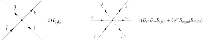
Figure 2. Interaction vertices for the phase-space field. p¯ldenotes the momentum carried by the particle which propagates along the ¯l-leg.
¯
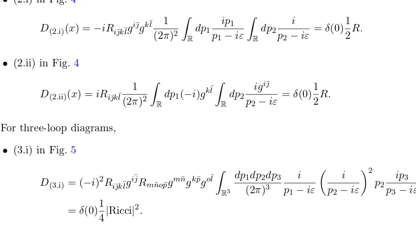
Figure 3. Interaction vertices for the auxiliary field with the phase-space field.
As we want only to evaluate diagrams up to order κ−2, we only need to consider a few
Figure 4. Two-loop vacuum diagrams, (2.i) left and (2.ii) right.
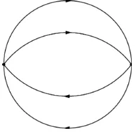
Figure 5. Three-loop vacuum diagram (3.i).
where GL is the set of bubble diagrams with L loops, Aut(Γ) is the subgroup of the group of
automorphisms of Γ that maps vertices to vertices of the same type and oriented propagators to oriented propagators of the same type (which start and end at the same vertices), |Aut(Γ)|= #Aut(Γ) is also known assymmetry factor, andDΓ(x) is the evaluation of the Feynman diagram.
The evaluation of each diagramDΓ(x) follows from the Feynman rules in momentum space:
to each line we associate its corresponding propagator (Fig. 1), to each vertex we associate its corresponding numerical factor (Figs. 2 and 3), we impose momentum conservation at each vertex and integrate over each undetermined momentumRR
dp
2π. There are two types of integrals that appear in the evaluation of bubble diagrams
lim
Each vacuum diagram is proportional to the Dirac deltaδ(0), or the “total length” ofR, because
the calculation in the momentum space yields the total vacuum energy in R. As we are just
interested in the vacuum energydensity, we will divide out by infinite total length of the (0 + 1)-spacetime, R. Thus, in order to determine E′
0(x) up to three loops, we use equation (11). The
Figure 6. Three-loop vacuum diagram (3.ii).
Figure 7. Three-loop vacuum diagram (3.iii).
• (3.ii) in Fig. 6
D(3.ii) = (−i)2Ri¯k¯lRi¯k¯l
Z
R4
dp1dp2dp3dp4
(2π)4 δ(p1+p3−p2−p4)p1p2
× i
p1−iε
i p2−iε
i p3−iε
i p4−iε
=−|Riemann|2
Z
R3
dp1dp2dp3
(2π)3
1
(p3−iε)[(p1+p3−p2)−iε]
=−|Riemann|2
Z
R3
dl1dl2dl3
(2π)3
i
(l1−iε)(l2−iε)
=δ(0)1
4|Riemann|
2,
wherel1 =p1+p2−p3,l2 =p3 and l3=p2.
• (3.iii) in Fig.7
D(3.iii)= −i 4
∆R+ 3
2 3|Ricci|
2+1
3|Riemann|
2
× lim ε→0+
Z
R3
dp1dp2dp3
(2π)3
i p1−iε
i p2−iε
ip3
p3
=δ(0) 1
16 ∆R+ 2|Ricci|
2+|Riemann|2.
• (3.iv) in Fig. 8. Similarly to (3.i)
D(3.iv) =δ(0)
1 4|Ricci|
2.
• (3.v) in Fig.8
D(3.v)=δ(0)
1 4|Ricci|
Figure 8. Three-loop vacuum diagrams with auxiliary field, (3.iv) left and (3.v) right.
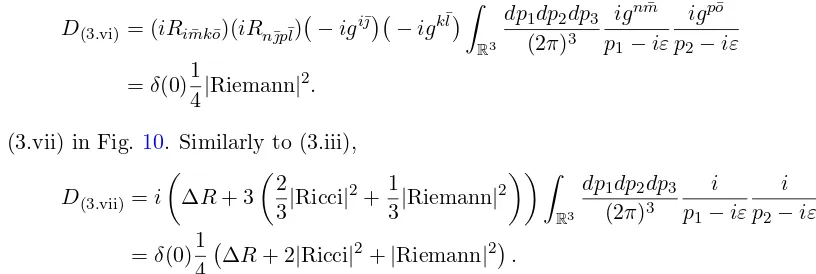
Figure 9. Three-loop vacuum diagram with auxiliary field (3.vi).
Figure 10. Three-loop vacuum diagram with auxiliary field (3.vii).
• (3.vi) in Fig. 9. Similarly to (3.ii),
D(3.vi) = (iRimk¯ o¯)(iRnp¯¯l) −igi¯
−igk¯l Z
R3
dp1dp2dp3
(2π)3
ignm¯
p1−iε
igp¯o p2−iε
=δ(0)1
4|Riemann|
2.
• (3.vii) in Fig.10. Similarly to (3.iii),
D(3.vii)=i
∆R+ 3
2 3|Ricci|
2+1
3|Riemann|
2 Z
R3
dp1dp2dp3
(2π)3
i p1−iε
i p2−iε
=δ(0)1
4 ∆R+ 2|Ricci|
2+
|Riemann|2.
Finally, including the symmetry factors of each diagram, and summing them as in equa-tion (11), yields the vacuum energy density associated to the semiclassical vacuum state localized atx∈M,
E0′(x) = 1 2κR+
1
96κ2 5∆R+ 42|Ricci|
2+ 17|Riemann|2+O
1 κ3
. (12)
Thus, comparing equation (12) with the equivalent result in geometric quantization (7), yields different vacuum energy densities E0(x) 6= E0′(x), despite the fact that the leading terms are
5
Conclusion
We have shown how the K¨ahler–Einstein metrics appear naturally in the classical limit of K¨ahler quantization. In geometric quantization, identifying semiclassical vacuum states with coherent states allows us to define balanced metrics as those metrics which yield constant semiclassical vacuum energy (for constant classical Hamiltonian). In the Berezin’s approach to deformation quantization, the unit element of the noncommutative algebra C∞(M)[[κ−1]] is the constant function, if and only if the metric is balanced. Also in path integral quantization, requiring the semiclassical vacuum energy to be constant yields a metric that is K¨ahler–Einstein in the classical limit.
Strictly speaking, the metrics that appear in path integral quantization are not balanced. This is due to a different choice of vacuum states in the path integral formalism; thus, for each choice of moduli spaces of semiclassical vacua one can define differentgeneralized balanced metrics. It would be interesting to study the properties exhibited by this general class of metrics. For instance, it is especially interesting to understand how introducing quantum corrections to the K¨ahler potential deforms the moduli of semiclassical vacua [16].
Another interesting problem would be to understand balanced metrics in vector bundles within the framework of K¨ahler quantization. Also, one could explicitly construct special La-grangian submanifolds in Calabi–Yau threefolds, and give ageometric quantization formulation of the Bressler–Soilbeman conjecture [5] (which conjectures a correspondence of the Fukaya category with a certain category of holonomic modules over the quantized algebra of functions). A final motivation for future research comes from the fact that the geometric objects explored in this paper appear in the large volume limit of string theory compactifications. We have shown how these objects can be explicitly constructed in the semiclassical limit of geometric quantization; one would expect that different areas of string theory, such as Matrix theory, black holes, and Calabi–Yau compactification theory [3,7,13,14], where the quantized algebra of functions plays a special role, could be understood better through a deeper study of the ideas explored here.
Acknowledgements
It is a pleasure to thank T. Banks, E. Diaconescu, M. Douglas, R. Karp, S. Klevtsov, and specially the author’s advisor G. Moore, for valuable discussions. We would like to thank as well G. Moore and G. Torroba for their comments on the manuscript, and J. Nannarone for kind encouragement and support. This work was supported by DOE grant DE-FG02-96ER40949.
References
[1] Alvarez-Gaum´e L., Freedman D.Z., Mukhi S., The background field method and the ultraviolet structure of the supersymmetric nonlinearσ-model,Ann. Physics134(1981), 85–109.
[2] Axelrod S., Della Pietra S., Witten E., Geometric quantization of Chern–Simons gauge theory,J. Differential Geom.33(1991), 787–902.
[3] Banks T., Fischler W., Shenker S.H., Susskind L., M theory as a matrix model: a conjecture,Phys. Rev. D
55(1997), 5112–5128,hep-th/9610043.
[4] Bordemann M., Meinrenken E., Schlichenmaier M., Toeplitz quantization of K¨ahler manifolds andgl(N), N→ ∞limits,Comm. Math. Phys.165(1994), 281–296,hep-th/9309134.
[5] Bressler P., Soibelman Y., Mirror symmetry and deformation quantization,hep-th/0202128.
[6] Cattaneo A.S., Felder G., A path integral approach to the Kontsevich quantization formula,Comm. Math. Phys.212(2000), 591–611,math.QA/9902090.
[7] Cornalba L., Taylor W., Holomorphic curves from matrices, Nuclear Phys. B 536 (1998), 513–552,
[8] Donaldson S.K., Scalar curvature and projective embeddings. I,J. Differential Geom.59(2001), 479–522.
[9] Donaldson S.K., Some numerical results in complex differential geometry, Pure Appl. Math. Q. 5(2009),
571–618,math.DG/0512625.
[10] Douglas M.R., Karp R.L., Lukic S., Reinbacher R., Numerical solution to the hermitian Yang–Mills equation on the Fermat quintic,J. High Energy Phys.2007(2007), no. 12, 083, 24 pages,hep-th/0606261.
[11] Douglas M.R., Karp R.L., Lukic S., Reinbacher R., Numerical Calabi–Yau metrics, J. Math. Phys. 49
(2008), 032302, 19 pages,hep-th/0612075.
[12] Elitzur S., Moore G.W., Schwimmer A., Seiberg N., Remarks on the canonical quantization of the Chern– Simons–Witten theory,Nuclear Phys. B326(1989), 108–134.
[13] Gaiotto D., Simons A., Strominger A., Yin X., D0-branes in black hole attractors, J. High Energy Phys.
2006(2006), no. 3, 019, 24 pages,hep-th/0412179.
[14] Kachru S., Lawrence A.E., Silverstein E., On the matrix description of Calabi–Yau compactifications,Phys. Rev. Lett.80(1998), 2996–2999,hep-th/9712223.
[15] Kapustin A., Topological strings on noncommutative manifolds,Int. J. Geom. Methods Mod. Phys.1(2004),
49–81,hep-th/0310057.
[16] Karabegov A.V., Deformation quantizations with separation of variables on a K¨ahler manifold, Comm. Math. Phys.180(1996), 745–755,hep-th/9508013.
[17] Kontsevich M., Deformation quantization of Poisson manifolds. I, Lett. Math. Phys.66 (2003), 157–216,
q-alg/9709040.
[18] Lu Z., On the lower order terms of the asymptotic expansion of Tian–Yau–Zelditch, Amer. J. Math.122
(2000), 235–273,math.DG/9811126.
[19] Rawnsley J.H., Coherent states and K¨ahler manifolds,Quart. J. Math. Oxford Ser. (2)28(1977), no. 112,
403–415.
[20] Reshetikhin N., Takhtajan L.A., Deformation quantization of K¨ahler manifolds, in L.D. Faddeev’s Seminar on Mathematical Physics,Amer. Math. Soc. Transl. Ser. 2, Vol. 201, Amer. Math. Soc., Providence, RI, 2000, 257–276,math.QA/9907171.
[21] Seiberg N., Witten E., String theory and noncommutative geometry, J. High Energy Phys.1999(1999),
no. 9, 032, 93 pages,hep-th/9908142.
[22] Souriau J.M., Structure of dynamical systems. A symplectic view of physics, Progress in Mathematics, Vol. 149, Birkh¨auser Boston, Inc., Boston, MA, 1997.
[23] Zelditch S., Szeg¨o kernels and a theorem of Tian,Internat. Math. Res. Notices1998(1998), no. 6, 317–331,