Hybrid dynamical systems vs. ordinary differential
equations: Examples of ”pathological” behavior
Elena Litsyn
∗Yurii V. Nepomnyashchikh
†Arcady Ponosov
‡Keywords. Stabilization, hybrid feedback control, functional differential equations.
AMS (MOS) subject classification. 93D15
1
Introduction
We study the following scalar equation
¨
ξ+ξ =u. (1)
Here, the control u depends on the variable ξ. This is a controlled harmonic oscillator in which the external forceu is allowed to depend only on the displacement ξ, but not on the velocity ˙ξ of the pendulum.
Equation (1) with the constraint u(ξ) is equivalent to the following controlled linear system
˙
ξ=η,
˙
η=−ξ+u, y=ξ
(2)
with a controlu=u(y). Here u again depends only on the output y=ξ.
It can be shown (see e.g. [1]) that there is no output feedback control of the formu=f(ξ) =
f(ξ(t)) that makes the system (2) asymptotically stable. Therefore, it was suggested in [1] to use
hybrid feedback controls(abbr. HFC), which indeed can stabilize the system (2).
The idea used in [1] can be roughly described as follows. We incorporate a discrete device (an automaton) into the considered system ( a plant). The device is able to switch on and off certain control functions at certain instances. The time interval between two consecutive switchings depends on the last observation of ξ. As it was demonstrated in [1], careful choice of design procedure and switching instances provides asymptotic stability of the system (2). The discrete nature of hybrid outputs makes their practical implementation simpler.
More results on stabilization of linear and nonlinear systems via HFC with a finite number of automata’s locations are available (see e.g. [2], [3], [4], [5], [6], [8], [10]). In [7] it was proved that it is possible to stabilize an arbitrary linear system by using HFC with infinitely many locations.
∗Department of Mathematics, Ben-Gurion University of the Negev, Beer-Sheva, ISRAEL; Partially supported
by the Ministry of Science and the Ministry of Absorption, Center for Absorption in Science, Israel. Email: [email protected]
†Department of Mechanics & Mathematics, Perm State University, Bukirev str. 15, 614600 Perm, RUSSIA;
Supported by the Norwegian Research Council. Email: [email protected]
In this paper we show that the dynamics of solutions x(t) of the system (2) which is controlled by the hybrid output designed in [1, Example 5.2], is quite erratic (see Figure 1). Trajectories’ be-havior indicates that the observed dynamics cannot be described by ”classical” dynamical systems defined by ordinary differential equations. We suspect that this dynamics stems from differential equations with time lags, where the delay functions depend on solutions. We are planning to study this problem in the future.
The whole dynamics of hybrid dynamical systems is given by thetriplet (x(t), q(t), τ(t)), where
q(t) is the present location of the automaton, and τ(t) is the time remaining untill the next transition instance. We are interested here in dynamic properties of the first, most important, component,x(t), which describes the plant. To be able to ”track down” x(t) we need however to study the dynamics of the whole triplet.
x (t)1
x (t)2
x (t)i
h
x
x (t)1
x (t)2
x (t)1
h
x
x (t)1 x (t)1
x (t)2 x (t)2
x (t)i x (t)2
h
x
x (t)2
x (t)1
Figure 1
2
Main results
We consider the controlled harmonic oscillator (2) assuming that u is a specific HFC designed in [1, Example 5.2]. This control procedure provides asymptotic stability of the zero solution of the system. For the sake of brevity we, as in [8], denote this HFC by u = A(δ), where δ is to be specified.
The HFC A(δ) is given by the following diagram
x(t) 0r T =- - d
u = 3- x
q
dT =d
u = 0
q _
q
+T =d
u = 0
x(t)<0
x(t)<0
x(t)<0 x(t)
0
r
x(t) 0
r
p
4
Figure 2
The automaton has 3 locations called q+, q− and qd, and the values of T indicate the time of
staying in the respective locations.
2δ. Our alteration is technical and does not influence the main results.
As was already mentioned the dynamics of the system (1) governed by the HFC, u=A(δ) is a triplet (x(t), q(t), τ(t)). However it is clear that the value τ(t) is uniquely determined by the value q(s), where s≤t is the moment of the last observation. In particular,τ(0) is a function of
q(0). In what follows we fix an arbitrary initial locationq(0) (as we will show, all the results below are independent of the choice of q(0)). Then, given an initial value x(0), the trajectory x(t) is uniquely defined, so that we, at least formally, can set up a single functional-differential equation
˙
x=F x=F(q(0))x (3)
for all x(t) (see details in [7] and [9]). We are interested in the dynamics of this equation.
We start with some technical remarks. Consider a solution x(t) = (ξ(t), η(t)) of the equation (3), i.e. of the system (2) governed by the HFC u =A(δ) with q(0) fixed. The trajectoryx(t) is assumed to start at x(0)6= 0.
We will use polar coordinates in the plane, so that any solution x(t) = (ξ(t), η(t)) of (3) is described by the (uniquely defined) pair of functions r: [0,∞)→[0,∞), ϕ: [0,∞)→R/(2πZ), whereξ(t) =r(t) cosϕ(t), η(t) =r(t) sinϕ(t).
In what follows we assume that the function ϕ takes on values from the interval (−π, π].
Within any interval S = (s1, s2) ⊂ [0,∞), where no change of locations occurs, the solution
x(t) satisfies one of the following systems of differential equations:
(q(t) =q+, t∈S ) ∨ (q(t) =q−, t∈S ) =⇒ (
˙
r r = 0
˙
ϕ =−1, (4)
(q(t) =qd, t ∈S) =⇒
(r˙
r =−32 sin 2ϕ ˙
ϕ=−1−3 cos2
ϕ. (5)
Theorem 1 There exist δ > 0, t∗ > 0 and two distinct initial states x1(0), x2(0), for which the corresponding solutions x1(t) and x2(t) to (2) governed by the HFC u = A(δ) coincide for t ≥ t∗, i.e. x1(t) = x2(t), t ≥ t∗. Moreover, in this case the ”true” hybrid trajectories H1(t) =
(x1(t), q1(t), τ1(t)) and H2(t) = (x2(t), q2(t), τ2(t)) coincide for t≥t∗, too.
Proof. We use equations (4) and (5) to derive estimates for solutions of (3) (i. e. of the system (2) with u=A(δ)). Assume that s1, s2 ∈[0,∞),s1 ≤s2.
1) If either q(·)≡q+, or q(·)≡q+ on [s1, s2] , then
ϕ(s1)−ϕ(s2) =s2−s1, (6)
r(s1) =r(s2). (7)
2) If q(·)≡qd on [s1, s2] and ϕ([s1, s2])⊂(−π/2, π/2), then
s2−s1 = 1
2 arctan
tanϕ(s1)
2 −arctan
tanϕ(s2) 2
!
(8)
r(s2)
r(s1) = v u u t
1 + 3 cos2ϕ(s1)
Put Td=π/4−δ as the time of stay in the location qd. Let ¯t be the moment of switching to
the locationqd. Then ¯t+Td is the moment of switching fromqd to another location. We define a
functionθ : [π/2−δ, π/2]→R by θ(ϕ) =ϕ(¯t+Td), ifϕ =ϕ(¯t). Due to (8),
θ(ϕ) = −arctan
2·cot
arctantanϕ 2 + 2δ
, ϕ ∈ π
2 −δ,
π
2
, (10)
so thatθ(ϕ) is well-defined for sufficiently small δ, namely for those satisfying
θ
π 2
−θ
π 2 −δ
> δ. (11)
We also define β : [π/2−δ, π/2]→R by
β(ϕ) = v u u t
1 + 3 cos2ϕ
1 + 3 cos2θ(ϕ). (12)
From (11) and continuity of the functionθ, it is easy to derive the existence ofψ1, ψ2 ∈R, for which
π
2 −δ < ψ1 < ψ2 <
π
2, θ(ψ2)−θ(ψ1) =δ. (13)
From now on we fix a positive and sufficiently small δ as well as two constants ψi satisfying
(13).
We pick two different trajectories x1(t), x2(t) being the ”shadows” of the ”true” hybrid tra-jectories
Hi(t) = (xi(t), qi(t), τi(t)), i= 1,2,
We assume that at t = t0 ≥ 0 the automaton either switches from q− to qd, or keeps staying in q−. In polar coordinates one has
ϕ1(t0) =ψ1+δ, r1(t0) =r0 >0, ϕ2(t0) = ψ2, r2(t0) =r0 β(ψ1)
β(ψ2). (14)
An example of such a situation is given byq(0) =q−andt0 =nδ, wherenis a nonnegative integer satisfying nδ < π
2 −δ.
Clearly, r2(t0)< r1(t0) (the function β is strictly increasing).
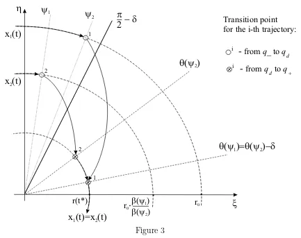
The two observations below can easily be derived from (13). See also Figure 3.
1) In the case of the trajectory x1(t), the automaton keeps staying in the location q− near t=t0; i.e., H1(t) = (x1(t), q−, δ) fort0 < t < t0+δ. The first transition to the location qd occurs
att=t0+δ; i.e., H1(t0+δ) = (x1(t0+δ), qd, Td).
2) In the case of the trajectory x2(t), the automaton switches from q− to qd at t = t0; i.e., H2(t0) = (x2(t0), qd, Td). At the moment t =t0+Td the automaton switches from qd toq+; i.e., H2(t0+Td) = (x1(t0+Td), q+, δ).
These observations imply that
qi(t∗) = q+, τi(t∗) =δ, i= 1,2, (15)
wheret∗ =t0+π
4 =t0+Td+δ.
At the same time, from (6), (14) and the observations above it follows that
ϕ1(t0+δ) = (ψ1+δ)−δ=ψ1, ϕ1(t∗) =θ(ψ1),
Thus, it is shown that
ϕ1(t∗) =ϕ2(t∗). (17)
Since ϕi is strictly monotone on [t0, t∗], there exist functions ρi (i= 1,2), defined on the set Di =ϕ−
1
i ([t0, t∗]) and satisfying
ri(t) =ρi(ϕi(t)). (18)
h
x (t)
1x (t)
2y
1y
2
p
2
- - d
1
2
1 2
q(y )
2q(y )=q(y )-d
1 2r(t*)
r0
b(y )1
b(y )2
r0
x (t)=x (t)
1 2.
.
.
i
i
-
fromq_toqd
-
fromq toqd +
Transition point for the i-th trajectory:
x
[image:5.595.90.523.157.500.2].
Figure 3 Then (7), (9), (12), (16) imply
r1(t∗) =ρ1(ϕ1(t∗)) =ρ1(θ(ψ1)) =β(ψ1)ρ1(ψ1) =β(ψ1)r0,
r2(t∗) =r2(t0+T
d) =ρ2(θ(ψ2)) = β(ψ2)ρ2(ψ2) =β(ψ2)r2(t0).
From this and (14) one gets
r1(t∗) =r2(t∗). (19)
Now, (17), (19) imply x1(t∗) = x2(t∗). Taking this and (15) into account one observes that H1(t) =H2(t) fort ≥t∗ and, in particular, x1(t) =x2(t) for t≥t∗.
Theorem 2 There exist positive δ, ε, t∗, t∗∗ (t∗ < t∗∗) and distinct initial states x1(0), x2(0), for which the corresponding solutions x1(t) andx2(t) to (2) governed by the HFC u=A(δ)satisfy the following properties
1) x1(t) =x2(t) for t∗ ≤t≤t∗∗,
2) x1(t)6=x2(t) for t∗−ε < t < t∗ and t∗∗< t < t∗∗+ε,
while for the ”true” hybrid trajectories H1(t) = (x1(t), q1(t), τ1(t))and H2(t) = (x2(t), q2(t), τ2(t))
one has
Proof. Putting again Td = π
4 we will use the same functions θ and β as in the course of the
proof of Theorem 1. Similar to (13) we fix sufficiently small δ > 0, µ > 0 and two constants ψ1
and ψ2, giving an increasing function β and relations
π
2 −δ < ψ1 < ψ2 <
π
2, θ(ψ2)−θ(ψ1) =δ+µ, 0< µ < ψ1+δ−
π
2. (20)
h
x (t)
1x (t)
2y
1y
2
p
2
- - d
1
2
1 2
q(y )
2q(y )=q(y )-d-m
1 2r0
b(y )1 b(y )2
r0
x (t)=x (t)
1 2.
.
i i
-
fromq_toqd
-
fromq toqd +
Transition point for the i-th trajectory:
x
x (t)
1x (t)
2p
2
- - d
-1 2
i
-
fromq toqd
+
1
-
x (t*)=x (t*)1 22
-
x (t**)=x (t**)1 2.
Figure 4
Consider two different trajectories x1(t), x2(t), t ≥ t0 > 0 of the system (2) governed by the HFCu=A(δ), for which (14) hold true. Assume that
q1(t0) =q−, τ1(t0) =µ, q2(t0) = qd, τ2(t0) =Td. (21)
Clearly, (20) and (21) imply
q1(t0+µ+δ) =qd, τ1(t0+µ+δ) =Td, q2(t0+Td) =q+, τ2(t0+Td) =δ, (22)
and hence
q1(t∗) =q+, τ1(t∗) =δ, q2(t∗) =q+, τ(t∗) =δ−µ, (23)
wheret∗ =t0+T
From (8), (14), (20), (23) it follows that
ϕ1(t0+δ+µ) =ψ1 +δ−δ=ψ1, ϕ1(t∗) =θ(ψ1),
ϕ2(t0+Td) =θ(ϕ2(t0)) =θ(ψ2), ϕ2(t∗) =θ(ψ2)−δ−µ=θ(ψ1).
(24)
Thus, the condition (17) is verified.
On the other hand, an argument similar to that used in the proof of Theorem 1 shows that
r1(t∗) =β(ψ1)r1(t0) r2(t∗) =r2(t0+T
d) =β(ψ2)r2(t0)
due to (7), (9), (12), (23), (24).
From this and (14) one easily derives (19).
Due to (22), q1(t∗−ε) =qd and q2(t∗−ε) =q+ for sufficiently smallε. This and (7) together
with (9) imply
r1(t)6=r2(t), t∗−ε < t < t∗. (25)
By (6), (7), (17), we have that (19) and (23) imply the existence of t∗∗> t∗, for which
x1(t) =x2(t) for t∗ ≤t≤t∗∗, (26)
and
ϕ1(t∗∗)∈[−π
2 −δ,−
π
2), τ1(t) =τ2(t) +µ for t
∗ ≤t≤t∗∗, q1(t∗∗) =q+, τ1(t∗∗) =µ, q2(t∗∗) =q
d, τ2(t∗∗) =Td.
The last four equalities say that in the case of the trajectoryx2(t) the automaton switches fromq+
toqdat time t=t∗∗, while in the case of the trajectory x1(t) switching occurs at time t=t∗∗+µ.
From (9) and (26) one obtains
H1(t)6=H2(t) for t∗ ≤t≤t∗∗
r1(t)6=r2(t) for t∗∗ < t < t∗∗+ε, (27)
for sufficiently smallε >0.
The relations (25) - (27) prove the theorem.
Theorem 3 . There exist δ >0 and two distinct initial states x1(0), x2(0), for which the corre-sponding solutions to (2) governed by the HFC u =A(δ) meet transversely at some time t∗ > 0. In other words, x1(t∗) = x2(t∗), x1(t)6=x1(t) for small |t−t∗| 6= 0, and the vectors x1˙ (t∗), x2˙ (t∗) are linearly independent.
Proof. As in the proof of theorem 2 let us fix sufficiently smallδ >0,µ >0 and some constants
ψ1, ψ2, so that the function β defined by (12) is increasing and (20) holds.
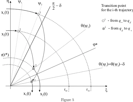
Consider two solutions x1(t), x2(t) of the system (2) governed by the HFC u = A(δ). The solutions are assumed to satisfy
ϕ1(t0) =ψ1+δ, r1(t0) =r01, ϕ2(t0) =ψ2, r2(t0) = r02< r01 (28)
h
x (t)
1x (t)
2y
1y
2
p
2
- - d
1
2 2
q(y )
2q(y )=q(y )-d
1 2r02 r01
.
.
i
i
-
fromq_toqd-
fromq toqd +
Transition point for the i-th trajectory:
x
r(t*)
1
x (t)
2x (t)
1 [image:8.595.87.518.67.396.2]j*
Figure 5
As in the proof of Theorem 1, the relations (28) imply that
ϕ1(t0+δ+Td) =θ(ψ1), ϕ2(t0+δ+Td) =θ(ψ2)−δ=θ(ψ1) +µ.
Moreover, using the second inequality in (5), the mean value theorem and (20), (28) one can easily show that
ϕ1(t0+Td)> ϕ2(t0+Td), ϕ1(t0+Td+δ)< ϕ2(t0 +Td+δ)
for sufficiently smallµ >0.
Due to the continuity of ϕi(t) there exists t∗ ∈(t0+Td, t0+Td+δ), for which (17) holds true.
We also putϕ∗ =ϕi(t∗).
Let ω : [π 2 −δ,
π
2]→R be a function defined by
ω(ψ1, ψ2) = s
1 + 3 cos2ψ1
1 + 3 cos2ψ2.
Puttingψi =ϕ(ti) and comparing the definition of ω with (9) we, as in Theorem 1, obtain
ρi(s2) ρi(s1)
=ω(s1, s2), s1, s2 ∈ϕi(I) (29)
being valid for any time interval I ⊂ [t0, t1], during which the automaton keeps staying in the locationqd. This applies to both of solutions x1(t) andx2(t), so that we may put ρ1 =ρ2 =ρ.
According to our calculations, neither t∗, nor ϕ∗ depends on r0i. This means that we can
always find a pair r01, r02, for which the following additional assumption holds:
According to (17) and (29),
r1(t∗) =ρ1(ϕ∗) =ω(ψ1, ϕ∗)r01,
r2(t∗) =r2(t0+T
d) =ρ2(θ(ψ2)) =ω(ψ2, θ(ψ2))r02,
so that (30) implies (19). From (17) and (19) it immediately follows that x1(t∗) = x2(t∗). Since r1(t) is strictly monotone and ρ2(t) is a constant in some neighbourhood Ot∗ of the point t∗, we see thatx1(t)6=x2(t) (∀t∈Ot∗\ {t∗}).
Finally, we observe that
q1(t∗) =q
d, q2(t∗) =q+. (31)
Put (ξ, η)T
=x1(t∗) =x2(t∗). Evidently, ξη 6= 0. Hence,
αx1˙ +βx2˙ = 0 α+β −α−4β 0
!
ξ η
! 6= 0
for |α|+|β| 6= 0. Thus, the velocity vectors are linearly independent, and the theorem is proved.
Acknowledgments. We would like to thank the anonymous referee for many valuable remarks which helped us to improve the paper.
References
[1] Z. Artstein, Example of stabilization with hybrid feedback, in Hybrid Systems III. Verifica-tion and Control. Springer-Verlag, Berlin, Lecture Notes in Computer Science., 1066 (1996), pp. 173–185.
[2] C. Benassi, A. Gavioli,Hybrid stabilization of planar linear systems with one-dimensional outputs, preprint, Dipartamenta di Matematica Pura e Applicata, Universita di Modena, Italy, August 1999.
[3] M. S. Branicky, Stability of Switched and Hybrid Systems, in Proc. 33rd IEEE Conf. Decision Control, Lake Buena Vista, FL (1994), pp. 3498-3503.
[4] M. S. Branicky, Studies in hybrid systems: modeling, analysis and control, Ph.D. thesis, Massachusetts Institute of Technology, Cambridge, 1995.
[5] D. Liberzon, Stabilizing a linear system with finite-state hybrid output feedback, The 7th IEEE Mediterranean Conference on Control and Automation (1999).
[6] D. Liberzon, A.S.Morse,Benchmark problems in stability and design of switched systems, preprint, March 1999.
[7] E. Litsyn, Yu.V. Nepomnyaschchikh, and A. Ponosov, Stabilization of linear differ-ential systems via hybrid feedback controls, accepted for publication in SIAM J. Control and Optimization (1999).
[9] E. Litsyn, Yu.V. Nepomnyaschchikh, and A. Ponosov,Uniform exponential stability of controlled quasilinear systems and functional differential equations,”Topics on Functional Differential and Difference Equations” T. Faria and P. Freitas Eds,Fields Institute Commu-nications(submitted for publication in 2000).