23 11
Article 02.1.6
Journal of Integer Sequences, Vol. 5 (2002), 2
3 6 1 47
The function
v
M
m
(
s
;
a, z
)
and some well-known
sequences
Aleksandar Petojevi´c
Aleja Marˇsala Tita 4/224000 Subotica Yugoslavia
Email address: [email protected]
Abstract
In this paper we define the functionvMm(s;a, z), and we study the special cases1Mm(s;a, z)
and nM−1(1; 1, n+ 1). We prove some new equivalents of Kurepa’s hypothesis for the left
factorial. Also, we present a generalization of the alternating factorial numbers.
1
Introduction
Studying the Kurepa function
K(z) = !z=
Z +∞
0
tz−1
t−1 e −t
dt (Rez >0),
G. V. Milovanovi´c gave a generalization of the function
Mm(z) =
Z +∞
0
tz+m−Q m(t;z)
(t−1)m+1 e
−t
dt (Rez >−(m+ 1)),
where the polynomialsQm(t;z), m=−1,0,1,2, ... are given by
Q−1(t;z) = 0 Qm(t;z) =
m
X
k=0
µ
m+z k
(t−1)k.
The function {Mm(z)}+
∞
m=−1 has the integral representation
Mm(z) =
z(z+ 1)· · ·(z+m)
m!
Z 1
0
ξz−1
(1−ξ)me(1−ξ)/ξ
Γ³z,1−ξ ξ
´
dξ,
where Γ(z, x), the incomplete gamma function, is defined by
Γ(z, x) =
Z +∞
x
tz−1
e−t
dt. (1)
Special cases include
M−1(z) = Γ(z) and M0(z) =K(z), (2) where Γ(z) is the gamma function
Γ(z) =
Z +∞
0
tz−1
e−t
dt.
The numbersMm(n) were introduced by Milovanovi´c [10] and Milovanovi´c and Petojevi´c
[11]. For non-negative integers n, m∈N the following identities hold:
Mm(0) = 0, Mm(n) = n−1
X
i=0
(−1)i
i!
n−1
X
k=i
k!
µ
m+n k+m+ 1
.
For the numbersMm(n) the following relations hold:
Mm(n+ 1) = n! + m
X
ν=0
Mν(n),
lim
n→+∞
Mν(n)
Mν−1(n)
= 1,
lim
n→+∞
Mm(n)
(n−1)! = 1. The generating function of the numbers{Mm(n)}+
∞
n=0 is given by
1
m!
¡
Am(x)ex
−1
(Ei (1)−Ei (1−x) +Bm(x)ex−Cm(x))
¢
=
+∞
X
n=0
Mm(n)
xn
n!
whereAm(x), Bm(x), and Cm(x) are polynomials defined as follows:
Am(x)
m! =
m X k=0 µ m k 
(x−1)k
k! ,
Bm(x)
m! =
m−1
X
ν=0
Ãm−ν
X
k=1
µ
m k+ν
(−1)k−1
k
k−1
X
j=0
(−1)j
j!
!
(x−1)ν
ν! ,
Cm(x)
m! =
m−1
X
j=0
à j X
ν=0
(−1)ν
µ
j ν
¶ m X
k=j+1
(−1)k−1
k−ν
µ
m k
¶!
(x−1)j
Here Ei (x) is the exponential integral defined by
Ei (x) = p.v.
Z x
−∞
et
t dt (x >0). (3)
In this paper, we give a generalization of the function Mm(z) which we denote as vMm(s;a, z). These generalization are of interest because its special cases include:
1M1(1; 1, n+ 1) = n!,
1M0(1; 1, n) = !n,
nM−1(1; 1, n+ 1) = An.
where n!, !n, and An are the right factorial numbers (sequence A000142 in [17]), the left
factorial numbers(sequence A003422 in [17]) and thealternating factorial numbers(sequence A005165 in [17]), respectively. They are defined as follows:
0! = 1, n! =n·(n−1)!; !0 = 0, !n=
n−1
X
k=0
k! and An = n
X
k=1
(−1)n−k
k!. (4)
2
Definitions
We now introduce a generalization of the functionMm(z).
Definition 1 For m = −1,0,1,2, ..., and Rez > v −m −2 the function vMm(s;a, z) is
defined by
vMm(s;a, z) =
=
v
X
k=1
(−1)2v+1−k
Γ(m+z+ 2−k)
Γ(z+ 1−k)Γ(m+ 2) L[s; 2F1(a, k−z, m+ 2,1−t)],
where v is a positive integer, and s, a, z are complex variables.
The hypergeometric function 2F1(a, b;c, x) is defined by the series
2F1(a, b, c;x) =
∞
X
n=0
(a)n(b)n
(c)n
xn
n! (|x|<1),
and has the integral representation
2F1(a, b, c;x) =
Γ(c) Γ(b)Γ(c−b)
Z 1
0
tb−1
(1−t)c−b−1
(1−tx)−a
in thex plane cut along the real axis from 1 to ∞, if Rec >Reb >0. The symbols (z)n and L[s;F(t)] represent the Pochhammer symbol
(z)n=
Γ(z+n) Γ(z) , and Laplace transform
L[s;F(t)] =
Z ∞
0
e−st
[image:4.612.80.546.232.351.2]F(t)dt.
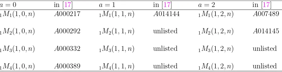
Table 1: The numbers 1Mm(1;a, n) form= 1,2,3,4 and a= 0,1,2
a= 0 in [17] a= 1 in [17] a= 2 in [17]
1M1(1,0, n) A000217 1M1(1,1, n) A014144 1M1(1,2, n) A007489
1M2(1,0, n) A000292 1M2(1,1, n) unlisted 1M2(1,2, n) A014145
1M3(1,0, n) A000332 1M3(1,1, n) unlisted 1M3(1,2, n) unlisted
1M4(1,0, n) A000389 1M4(1,1, n) unlisted 1M4(1,2, n) unlisted
The term “unlisted” in Table 1 means that the sequence cannot currently be found in Sloane’s on-line encyclopedia of integer sequences[17].
Lemma 1 Let m =−1,0,1,2, . . . . Then
1Mm(1; 1, z) =Mm(z).
Proof. The proof presented here is due to Professor G. V. Milovanovi´c. Since
(k+m+ 1)! = (m+ 1)!(m+ 2)k and (1−z)k=
(−1)kΓ(z)
Γ(z−k) , we have
µ
m+z k+m+ 1
= Γ(m+z+ 1)
Γ(z−k)(k+m+ 1)! =
Γ(m+z+ 1) Γ(z)(m+ 1)! ·
(1−z)k(−1)k
(m+ 2)k
,
so that
tz+m−Q m(t;z)
(t−1)m+1 = +∞
X
k=0
µ
m+z k+m+ 1
(t−1)k (|t−1|<1)
= Γ(m+z+ 1) Γ(z)(m+ 1)!
+∞
X
k=0
(1−z)k(1)k
(m+ 2)k
·(1−t) k
k!
= Γ(m+z+ 1)
3
The function
1M
m(
s
;
a, z
)
3.1
The numbers
{
1M
m(1;
−
n, r
)
}
+∞
r=0
+∞
n=0
+∞
m=−1
We have
1Mm(1;−n, z) =
Γ(m+z+ 1)
Γ(z)Γ(m+ 2) L[1;2F1(−n,1−z, m+ 2; 1−t)], starting with the polynomials
∞
X
k=0
µ
m+z k+m+ 1
¶µ
n k
(1−t)k, n ∈N.
Since
(−n)k = (−1)k
n! (n−k)! we have
∞
X
k=0
µ
m+z k+m+ 1
¶µ
n k
(1−t)k = Γ(m+z+ 1)
Γ(z)Γ(m+ 2)2F1(−n,1−z, m+ 2; 1−t) (5)
or, by continuation,
=πcosecπz
Z 1
0
ξ1−z
(1−ξ)m+z+1¡
1−(1−t)ξ¢n
dξ.
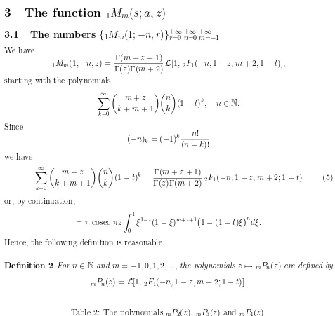
Hence, the following definition is reasonable.
Definition 2 For n ∈Nand m =−1,0,1,2, ..., the polynomials z 7→mPn(z) are defined by
[image:5.612.73.550.62.513.2]mPn(z) = L[1; 2F1(−n,1−z, m+ 2; 1−t)].
Table 2: The polynomials mP2(z),mP3(z) andmP4(z)
m mP2(z) mP3(z) mP4(z)
−1 12z2− 3
2z+ 2 −
1 3z3+
7 2z2−
49 6z+ 6
3 8z4−
61 12z3 +
193 8 z2−
0 16z2− 1 2z+
4
3 −
1 12z
3+z2− 29 12z+
5
2 −
509 12z+ 24
1 1
12z 2−1
4z+ 7
6 −
1 30z
3+ 9 20z
2− 67 60z+
17 10
The polynomialsmPn(z) can be expressed in terms of thederangement numbers (sequence
A000166 in [17])
Sk=k! k
X
ν=0
(−1)ν
Theorem 1 For m=−1,0,1,2, ... and n ∈N we have
mPn(z) =
µ
n+m+ 1
n
¶−1 ∞
X
k=0
µ
n+m+ 1
k+m+ 1
¶µ
z−1
k
(−1)kSk.
Proof. Using the relation (5) we have
mPn(z) =
Γ(z)Γ(m+ 2) Γ(m+z+ 1)
Z ∞
0
e−t ∞
X
k=0
µ
m+z k+m+ 1
¶µ
n k
(1−t)kdt
= Γ(z)(m+ 1)! Γ(m+z+ 1)
∞
X
k=0
Γ(m+z+ 1) Γ(z−k)(k+m+ 1)!
µ
n k
¶ Z ∞
0
e−t
(1−t)kdt
=
µ
n+m+ 1
n
¶−1 ∞
X
k=0
µ
n+m+ 1
k+m+ 1
¶µ
z−1
k
¶ Z ∞
0
e−t
(1−t)kdt.
Now use
L[s; (t+α)z−1 ] = e
αsΓ(z, αs)
sz (Res >0),
to obtain
mPn(z) =
µ
n+m+ 1
n
¶−1 ∞
X
k=0
µ
n+m+ 1
k+m+ 1
¶µ
z−1
k
(−1)kΓ(k+ 1,−1)
e .
Here Γ(z, x) is the incomplete gamma function. The result follows from
Γ(k+ 1,−1) =eSk.
Lemma 2 For n∈N we have
−1Pn(z) = 1 +n!
n
X
k=1
(−1)kS k
(n−k)! (k!)2
k
Y
i=1
(z−i).
Proof. Applying Theorem 1for m=−1, we have
−1Pn(z) =
n X k=0 µ n k ¶µ
z−1
k
(−1)kSk,
= 1 +n!
n
X
k=1
(−1)kS k
(n−k)!(k!)2
k
Y
i=1
Remark 1 Let the sequence Xn,k be defined by
Xn,k =
(
Yn, if n =k,
(n−k)Xn−1,k, if n > k,
where Yn= (n!)2. Since Xn,k = (n−k)! (k!)2 we have
−1Pn(z) = 1 +n!
n
X
k=1
(−1)kS k
Xn,k k
Y
i=1
(z−i).
Theorem 2 For m=−1,0,1,2, ... and n ∈N we have
mP0(z) = mP1(z) = 1
mPn(z) =
1
n+m+ 1 [(m+ 1)m−1Pn(z) +nmPn−1(z)], m >−1.
Proof. According to Theorem 1 we have
1
n+m+ 1[(m+ 1)m−1Pn(z) +nmPn−1(z)] =
(m+ 1)!n! (n+m+ 1)!
∞
X
k=0
µ
n+m k+m
¶µ
z−1
k
(−1)kSk+
+ (m+ 1)!n! (n+m+ 1)!
∞
X
k=0
µ
n+m k+m+ 1
¶µ
z−1
k
(−1)kSk.
The recurrence for mPn(z) now follows from
µ
a b
+
µ
a b+ 1
=
µ
a+ 1
b+ 1
.
Corollary 1 For m=−1,0,1,2, ... and n ∈N we have
1Mm(1;−n, z) =
n!z(z+ 1). . .(z+m) (n+m+ 1)!
∞
X
k=0
µ
n+m+ 1
k+m+ 1
¶µ
z−1
k
Corollary 2 For n∈N the result is as follows
1M−1(1;−n, z) = 1 +n!
n
X
k=1
(−1)kS k
(n−k)! (k!)2
k
Y
i=1
(z−i),
1Mm(1; 0, z) = 1Mm(1;−1, z) =
Γ(m+z+ 1) Γ(z)Γ(m+ 2),
1Mm(1;−n, z) =
1
n+m+ 1 ·[ (m+z)· 1Mm−1(1;−n, z) + + n· 1Mm(1;−n+ 1, z)], m >−1.
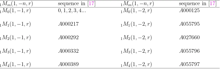
The numbers 1Mm(1;−n, r)
∞
[image:8.612.80.548.317.465.2]r=0 can now be evaluated recursively.
Table 3: The numbers1Mm(1;−n, r) for m= 0,1,2,3,4 and n = 1,2
1Mm(1,−n, r) sequence in [17] 1Mm(1,−n, r) sequence in [17]
1M0(1,−1, r) 0,1,2,3,4... 1M0(1,−2, r) A000125
1M1(1,−1, r) A000217 1M1(1,−2, r) A055795
1M2(1,−1, r) A000292 1M2(1,−2, r) A027660
1M3(1,−1, r) A000332 1M3(1,−2, r) A055796
1M4(1,−1, r) A000389 1M4(1,−2, r) A055797
3.2
The numbers
{
1M
m(1
/n
;
m
+ 2
, r
)
}
+∞
r=0
+∞
n=1
+∞
m=−1
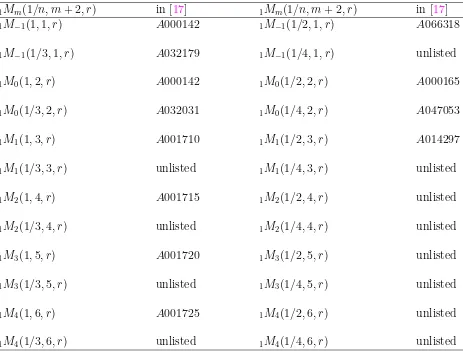
In Table 4 twelve well-known sequences from [17] are given. These sequences are special cases of the function vMm(s;a, r) for v = 1, s = 1/n, and a = m+ 2. The sequences have
the following common characteristic.
Lemma 3 For m=−1,0,1,2, ..., we have
1Mm(1/n;m+ 2, z) =
nzΓ(z+m+ 1)
(m+ 1)! .
Proof. Since
2F1(m+ 2,1−z, m+ 2,1−t) =tz
−1
we have
Table 4: The numbers 1Mm(1/n;m+ 2, r) form =−1,0,1,2,3,4 and n = 1,2,3,4
1Mm(1/n, m+ 2, r) in [17] 1Mm(1/n, m+ 2, r) in [17]
1M−1(1,1, r) A000142 1M−1(1/2,1, r) A066318
1M−1(1/3,1, r) A032179 1M−1(1/4,1, r) unlisted
1M0(1,2, r) A000142 1M0(1/2,2, r) A000165
1M0(1/3,2, r) A032031 1M0(1/4,2, r) A047053
1M1(1,3, r) A001710 1M1(1/2,3, r) A014297
1M1(1/3,3, r) unlisted 1M1(1/4,3, r) unlisted
1M2(1,4, r) A001715 1M2(1/2,4, r) unlisted
1M2(1/3,4, r) unlisted 1M2(1/4,4, r) unlisted
1M3(1,5, r) A001720 1M3(1/2,5, r) unlisted
1M3(1/3,5, r) unlisted 1M3(1/4,5, r) unlisted
1M4(1,6, r) A001725 1M4(1/2,6, r) unlisted
1M4(1/3,6, r) unlisted 1M4(1/4,6, r) unlisted
3.3
Some equivalents of Kurepa’s hypothesis
The special valuesM−1(z) = Γ(z) and M0(z) =K(z) given in (2) yield
1M−1(1,1, n+ 1) =n! and 1M0(1; 1, n) =!n (6) where n! and !n are the right factorial numbers and the left factorial numbers given in (4). The function n! and !n are linked by Kurepa’s hypothesis:
KH hypothesis. For n∈N\{1} we have
gcd( !n, n! ) = 2
where gcd(a, b) denotes the greatest common divisor of integers a and b.
This is listed as Problem B44 of Guy’s classic book [6]. In [8], it was proved that the KH is equivalent to the following assertion
The sequences an, bn, cn, dn and en (sequences A052169, A051398,
A051403, A002467 and A002720 in [17]) are defined as follows:
a2 = 1 a3 = 2 an = (n−2)an−1+ (n−3)an−2,
b3 = 2 bn = −(n−3)bn−1+ 2(n−2)
2,
c1 = 3 c2 = 8 cn = (n+ 2)(cn−1−cn−2),
d0 = 0 d1 = 1 dn = (n−1)(dn−1+dn−2),
e0 = 1 e1 = 2 en = 2nen−1−(n−1)
2e
n−2.
They are related to the left factorial function. For instance, let p > 3 be a prime number. Then
!p≡ −3ap−2 ≡ −bp ≡ −2cp−3 ≡dp−2 ≡ep−1 (mod p). We give the details for the last congruence.
Proof. Let
Lνn(x) =
n
X
k=0
Γ(ν+n+ 1) Γ(ν+k+ 1)
(−x)k
k!(n−k)!
be the Laguerre polynomials, and set L0
n(x) = Ln(x). Using the relation
¡p−1
k
¢
≡ (−1)k
(mod p), we have
Lp−1(x)≡ −(p−1)!
p−1
X
k=0
xk
k! (mod p).
Wilson’s theorem yields
!p≡ −Lp−1(−1) (mod p). The recurrence for Laguerre polynomials
(n+ 1)Lνn+1(x) = (ν+ 2n+ 1−x)Lnν(x)−(ν+n)Lνn−1(x),
for ν= 0, x=−1 produces
hp−1(p−1)!≡p (mod p), where
h1 = 2 h2 =
7
2 hn= 2hn−1−
n−1
n hn−2. The identity en=hnn! finally yields
4
The numbers
nM
−1(1; 1
, n
+ 1)
The special values
nM−1(1; 1, n+ 1) =An,
are the alternating factorial numbers given in (4). This sequence satisfies the recurrence relation
A0 = 0, A1 = (−1)n
−1
, An =−(n−1)An−1+nAn−2. These numbers can be expressed in terms of the gamma function as follows
An = n
X
k=1
(−1)n−k
Γ(k+ 1) =
Z ∞
0
e−x
à n X
k=1
(−1)n−k
xk
!
dx
=
Z ∞
0
e−xx
n+1−(−1)nx
x+ 1 dx.
The same relation is now used in order to define the function Az:
Definition 3 For every complex number z, Re z >0, the function Az is defined by
Az
def
=
Z ∞
0
e−xx
z+1−(−1)zx
x+ 1 dx.
The identity xz+1−(−1)zx
x+1 =x
z− xz
−(−1)z−1x
x+1 gives
Z ∞
0
e−xx
z+1−(−1)zx
x+ 1 dx=
Z ∞
0
e−x
xzdx−
Z ∞
0
e−xx
z −(−1)z−1
x x+ 1 dx,
i.e.,
Az = Γ(z+ 1)−Az−1. (7) This givesA0 = Γ(2)−A1 = 0 andA−1 = Γ(1)−A0 = 1.An inductive argument shows that
A−n, the residue of Az at the pole z =−n, is given by
res A−n= (−1)
n n−2
X
k=0
1
k!, n= 2,3,4, ...
The derivation employs the fact that Γ(z) is meromorphic with simple poles at z =−n and residue (−1)n/n! there.
The function Az can be expressed in terms of the exponential integral Ei (x) and the
incomplete gamma function Γ(z, x) by
Az =L[1;
tz+1−(−1)z
t+ 1 ] =eΓ(z+ 2)Γ(−z−1,1)−(−1)
4.1
The generating function for
A
n−1The total number of arrangements of a set with n elements (sequence A000522 in [17]) is defined (see [3], [5], [15] and [16]) by:
a0 = 1, an=nan−1+ 1, or an =n!
n
X
k=0
1
k!. (8)
The sequence {an} satisfies:
a0 = 1, a1 = 2, an= (n+ 1)an−1−(n−1)an−2, (9)
and
a0 = 1, an = n−1
X
k=0
µ
n k
(−1)n+1−k
(n+ 1−k)ak. (10)
Relation (9) comes from the theory of continued fractions and (10) follows directly from (8). We now establish a connection between the sequence {an} and the alternating factorial numbers An.
Lemma 4 Let a−1 = 1 and n ∈N\{1}. Then
An−1 =
n
X
k=0
µ
n k
(−1)n−k
ak−1.
Proof. Using (10) and induction on n we have
n! =
n
X
k=0
(−1)n−k
µ
n k
ak.
Inversion yields
an=n!− n
X
k=1
µ
n k−1
(−1)n+1−k
ak−1.
The relation¡n+1
k
¢
−¡n
k
¢
=¡ n
k−1
¢
, k≥1 produces
n+1
X
k=0
µ
n+ 1
k
(−1)n+1−k
ak−1+
n
X
k=0
µ
n k
(−1)n−k
ak−1 =n!.
The result now follows from (7).
Theorem 3 The exponential generating function for {An−1} is given by
g(x) =e1−x
[Ei(−1)−Ei(x−1) +e
−1
]−1 = ∞
X
n=2
An−1
xn
n!,
Proof. The expansion of the exponential integral
Ei(x) =γ+ ln(x) +
∞
X
k=1
xk
k·k!,
whereγ is Euler’s constant, appears in [1, p. 57, 5.1.10.]. The statement of the theorem can be written as
e[Ei(−1)−Ei(x−1) +e
−1 ] =e
"
−ln(x−1) + ∞
X
k=1
(−1)k−(x−1)k)
k·k!
#
=
= ∞
X
k=0
ak−1
xk
k!. (11)
Expand e−x
as a Taylor series to obtain
e−x =
∞
X
k=0
(−1)kx
k
k!.
Then
e1−x
[Ei(−1)−Ei(x−1) +e
−1
]−1 = ∞
X
k=0
ak−1
xk
k! ∞
X
k=0
(−1)kx
k
k! −1
= ∞
X
n=0
n
X
k=0
ak−1
xk
k!(−1)
n−k x
n−k
(n−k)!−1
= ∞
X
n=0
n
X
k=0
µ
n k
ak−1(−1)
n−kx
n
n! −1
= ∞
X
n=0
An−1
xn
n! −1.
By induction on n we get
Lemma 5 Let n ∈N. The function g(x) in Theorem 4.1 satisfies
g(n)(x) = d
dxg
(n−1)
(x) = (−1)n
"
g(x) + 1 +
n−1
X
k=0
k! (x−1)k+1
#
.
4.2
The AL hypothesis
In [6, p. 100] the following problem is given:
Problem B43. Are there infinitely many numbers n such that An−1 is a prime?
Here
An= n
X
k=1
(−1)n−k
k!.
If there is a value of n −1 such that n divides An−1, then n will divide Am−1 for all
m > n, and there would be only a finite number of prime values. The required condition for the existence of infinitely many numbers n such that An−1 is a prime may be expressed as follows:
AL hypothesis. For every prime number p
Ap−1 6≡0 (mod p),
holds.
Let p be a prime number and n, m ∈ N\{1}. It is not difficult to prove the following
results:
An−1 ≡ −1−
n
X
k=2
[k−1−(−1)n−k
]Γ(k) (mod n),
An−1 =
Γ(n+ 1)−1 +Pn−1
k=2[(−1)n
−k
n−k+ 1−(−1)n−k ]Γ(k)
n−1 ,
= 1−!n+ 2
n−1
X
k=1
Ak
= 3−!n−!(n−1)·2n+ 4
n
X
i=2
i−1
X
k=1
Ak.
n
X
k=1
m−1
X
i=0
(−1)i(Γ(k+ 1))m−i
Aik−1 =
Am
n, meven
Am n + 2
Pn−1
j=1 Amj , modd
,
Ap−1 =−
p
X
i=1
1 Γ(i) +p
p
X
i=1
ni(−1)i−1
Γ(i) , ni ∈N (i= 1,2, ...p)
5
Conclusions
The main contribution is to define the functionvMm(s;a, z) by which problems B43 and B44
are connected. The Kurepa hypothesis is an unsolved problem since 1971 and there seems to be no significant progress in solving it, apart from numerous equivalents, such as these in Section 3.3. Further details can be found in [7].
However, apart from n!, !n, and An, twenty-five more well-known sequences in [17] are
special cases of the function vMm(s;a, z). The first study of the function gave the author
the idea to find an algorithm for computing some special cases (Corollary 2 and Lemma 3) before solving the above mentioned problems.
The definition of the function vMm(s;a, z) suggest another method of studying the
func-tion by using the characteristics of the inverse Laplace transform.
Acknowledgements
I would like to thank the referee for the numerous comments and suggestions.
References
[1] M. Abramowitz, I. A. Stegun,Handbook of Mathematical Functions, Dover Publications, Inc. New York, 1965.
[2] C. Brezinski,History of Continued Fractions and Pad´e Approximants, Springer-Verlag, Berlin, 1991.
[3] P. J. Cameron, Sequences realized by oligomorphic permutation groups,J. Integer Se-quences 3(1) (2000), Article 00.1.5.
[4] L. Comtet,Advanced Combinatorics, Reidel, Dordrecht, 1974.
[5] J. M. Gandhi, On logarithmic numbers,Math. Student 31 (1963), 73–83.
[6] R. Guy, Unsolved Problems in Number Theory, Springer-Verlag, 1994.
[7] A. Ivi´c and ˇZ. Mijajlovi´c, On Kurepa problems in number theory, Publ. Inst. Math.
(N.S.) 57 (71) (1995), 19–28.
[8] -D. Kurepa, On the left factorial function !n, Math. Balkanica 1 (1971), 147–153.
[9] -D. Kurepa, Left factorial function in complex domain, Math. Balkanica 3 (1973), 297– 307.
[10] G. V. Milovanovi´c, A sequence of Kurepa’s functions,Sci. Rev. Ser. Sci. Eng.No.19–20 (1996), 137–146.
[12] O. Perron,Die Lehren von den Kettenb¨uchen, Chelsea Publishing Company, New York, 1954.
[13] A. Petojevi´c, On Kurepa’s hypothesis for left factorial, Filomat (Nis), 12 (1) (1998), 29–37.
[14] A. P. Prudnikov, Yu. A. Brychkov, and O. I. Marichev,Integrals and Series. Elementary Functions, Nauka, Moscow, 1981. (Russian)
[15] J. Riordan, An Introduction to Combinatorial Analysis, Wiley, 1958.
[16] D. Singh, The numbersL(m,n)and their relations with prepared Bernoulli and Eulerian numbers, Math. Student20 (1952), 66–70.
[17] N. J. A. Sloane,The On-Line Encyclopedia of Integer Sequences, published electronically at
http://www.research.att.com/~njas/sequences/
[18] H. S. Wilf, Generatingfunctionology, Academic Press, New York, 1990.
2000 Mathematics Subject Classification: Primary 11B83; Secondary 33C05, 44A10.
Keywords: left factorial, alternating factorial, hypergeometric function, Laplace transform
(Concerned with sequencesA000142,A003422,A005165,A000217,A014144,A007489,A000292,
A000332, A000389, A014145, A000166, A000125, A000217, A000389, A055795, A027660,
A055796, A055797, A032179, A032031, A001710, A001715, A001720, A001725, A066318,
A000165,A047053,A014297,A052169,A051398,A051403,A002467,A002720, andA000522.) Received March 21, 2002; revised version received August 14, 2002. Published in Journal of Integer Sequences August 31, 2002.