part I
1-1
What Macroeconomists Study
Why have some countries experienced rapid growth in incomes over the past century while others stay mired in poverty? Why do some countries have high rates of inflation while others maintain stable prices? Why do all countries expe-rience recessions and depressions—recurrent periods of falling incomes and ris-ing unemployment—and how can government policy reduce the frequency and severity of these episodes? Macroeconomics, the study of the economy as a whole, attempts to answer these and many related questions.
To appreciate the importance of macroeconomics, you need only read the newspaper or listen to the news. Every day you can see headlines such as IN-COME GROWTH SLOWS, FED MOVES TO COMBAT INFLATION, or STOCKS FALL AMID RECESSION FEARS. Although these macroeconomic events may seem abstract, they touch all of our lives. Business executives forecast-ing the demand for their products must guess how fast consumers’ incomes will grow. Senior citizens living on fixed incomes wonder how fast prices will rise. Recent college graduates looking for jobs hope that the economy will boom and that firms will be hiring.
Because the state of the economy affects everyone, macroeconomic issues play a central role in political debate.Voters are aware of how the economy is doing, and they know that government policy can affect the economy in powerful ways.As a result, the popularity of the incumbent president rises when the econ-omy is doing well and falls when it is doing poorly.
Macroeconomic issues are also at the center of world politics. In recent years, Europe has moved toward a common currency, many Asian countries have expe-rienced financial turmoil and capital flight, and the United States has financed large trade deficits by borrowing from abroad. When world leaders meet, these topics are often high on their agendas.
1
The Science of Macroeconomics
C H A P T E R
The whole of science is nothing more than the refinement of everyday thinking.
— Albert Einstein O N E
Although the job of making economic policy falls to world leaders, the job of explaining how the economy as a whole works falls to macroeconomists.Toward this end, macroeconomists collect data on incomes, prices, unemployment, and many other variables from different time periods and different countries. They then attempt to formulate general theories that help to explain these data. Like astronomers studying the evolution of stars or biologists studying the evolution of species, macroeconomists cannot conduct controlled experiments. Instead, they must make use of the data that history gives them. Macroeconomists ob-serve that economies differ from one another and that they change over time. These observations provide both the motivation for developing macroeconomic theories and the data for testing them.
To be sure, macroeconomics is a young and imperfect science. The macro-economist’s ability to predict the future course of economic events is no better than the meteorologist’s ability to predict next month’s weather. But, as you will see, macroeconomists do know quite a lot about how the economy works.This knowledge is useful both for explaining economic events and for formulating economic policy.
Every era has its own economic problems. In the 1970s, Presidents Richard Nixon, Gerald Ford, and Jimmy Carter all wrestled in vain with a rising rate of inflation. In the 1980s, inflation subsided, but Presidents Ronald Reagan and George Bush presided over large federal budget deficits. In the 1990s, with Pres-ident Bill Clinton in the Oval Office, the budget deficit shrank and even turned into a budget surplus, but federal taxes as a share of national income reached a historic high. So it was no surprise that when President George W. Bush moved into the White House in 2001, he put a tax cut high on his agenda. The basic principles of macroeconomics do not change from decade to decade, but the macroeconomist must apply these principles with flexibility and creativity to meet changing circumstances.
C A S E S T U D Y
The Historical Performance of the U.S. Economy
Economists use many types of data to measure the performance of an economy. Three macroeconomic variables are especially important: real gross domestic product (GDP), the inflation rate, and the unemployment rate.Real GDP mea-sures the total income of everyone in the economy (adjusted for the level of prices).The inflation ratemeasures how fast prices are rising.The unemploy-ment ratemeasures the fraction of the labor force that is out of work. Macro-economists study how these variables are determined, why they change over time, and how they interact with one another.
income allows us to enjoy a higher standard of living than our great-grand-parents did. Second, although real GDP rises in most years, this growth is not steady. There are repeated periods during which real GDP falls, the most dramatic instance being the early 1930s. Such periods are called reces-sionsif they are mild and depressionsif they are more severe. Not surpris-ingly, periods of declining income are associated with substantial economic hardship.
Figure 1-2 shows the U.S. inflation rate. You can see that inflation varies substantially. In the first half of the twentieth century, the inflation rate aver-aged only slightly above zero. Periods of falling prices, called deflation, were almost as common as periods of rising prices. In the past half century, inflation has been the norm. The inflation problem became most severe during the late 1970s, when prices rose at a rate of almost 10 percent per year. In recent years,
f i g u r e 1 - 1
World War I
Great Depression
World War II
Korean War
Vietnam War
First oil price shock Second oil price shock
1900 1910 1920 1930 1940 1950 1960 1970 1980 1990 30,000
35,000
20,000
10,000
5,000
3,000
Year
2000
Real GDP per person (1996 dollars)
Real GDP per Person in the U.S. Economy
Real GDP measures the total income of everyone in the economy, and real GDP per person measures the income of the average person in the economy. This figure shows that real GDP per person tends to grow over time and that this normal growth is sometimes interrupted by periods of declining income, called recessions or depressions.
Note:Real GDP is plotted here on a logarithmic scale. On such a scale, equal distances on the vertical axis represent equal percentagechanges. Thus, the distance between $5,000 and $10,000 (a 100 percent change) is the same as the distance between $10,000 and $20,000 (a 100 percent change).
the inflation rate has been about 2 or 3 percent per year, indicating that prices have been fairly stable.
Figure 1-3 shows the U.S. unemployment rate. Notice that there is always some unemployment in our economy. In addition, although there is no long-term trend, the amount of unemployment varies from year to year. Reces-sions and depresReces-sions are associated with unusually high unemployment. The highest rates of unemployment were reached during the Great Depression of the 1930s.
These three figures offer a glimpse at the history of the U.S. economy. In the chapters that follow, we first discuss how these variables are measured and then develop theories to explain how they behave.
f i g u r e 1 - 2
1900 30
25
20
15
10
5
0
−5
−10
−15
−20
Percent
Inflation
Deflation
1910
World War I
Great Depression
World War II
Korean War
Vietnam War
First oil price shock Second oil price shock
1920 1930 1940
Year
1950 1960 1970 1980 1990 2000
The Inflation Rate in the U.S. Economy
The inflation rate measures the percentage change in the average level of prices from the year before. When the inflation rate is above zero, prices are rising. When it is below zero, prices are falling. If the inflation rate declines but remains positive, prices are rising but at a slower rate.
Note: The inflation rate is measured here using the GDP deflator.
1-2
How Economists Think
Although economists often study politically charged issues, they try to address these issues with a scientist’s objectivity. Like any science, economics has its own set of tools—terminology, data, and a way of thinking—that can seem foreign and arcane to the layman.The best way to become familiar with these tools is to practice using them, and this book will afford you ample opportunity to do so.To make these tools less forbidding, however, let’s discuss a few of them here.
Theory as Model Building
Young children learn much about the world around them by playing with toy versions of real objects. For instance, they often put together models of cars, trains, or planes.These models are far from realistic, but the model-builder learns
f i g u r e 1 - 3
1900 25
20
15
10
5
0
Percent unemployed
1910
World War I
Great Depression
World War II
Korean War
Vietnam War
First oil price shock Second oil price shock
1920 1930 1940
Year
1950 1960 1970 1980 1990 2000
The Unemployment Rate in the U.S. Economy
The unemployment rate measures the percentage of people in the labor force who do not have jobs. This figure shows that the economy always has some unemployment and that the amount fluctuates from year to year.
a lot from them nonetheless.The model illustrates the essence of the real object it is designed to resemble.
Economists also use models to understand the world, but an economist’s model is more likely to be made of symbols and equations than plastic and glue. Economists build their “toy economies” to help explain economic variables, such as GDP, inflation, and unemployment. Economic models illustrate, often in mathematical terms, the relationships among the variables. They are useful be-cause they help us to dispense with irrelevant details and to focus on important connections.
Models have two kinds of variables: endogenous variables and exogenous variables.Endogenous variables are those variables that a model tries to ex-plain.Exogenous variablesare those variables that a model takes as given.The purpose of a model is to show how the exogenous variables affect the endoge-nous variables. In other words, as Figure 1-4 illustrates, exogeendoge-nous variables come from outside the model and serve as the model’s input, whereas endogenous variables are determined inside the model and are the model’s output.
To make these ideas more concrete, let’s review the most celebrated of all eco-nomic models—the model of supply and demand. Imagine that an economist were interested in figuring out what factors influence the price of pizza and the quantity of pizza sold. He or she would develop a model that described the be-havior of pizza buyers, the bebe-havior of pizza sellers, and their interaction in the market for pizza. For example, the economist supposes that the quantity of pizza demanded by consumers Qd depends on the price of pizza P and on aggregate income Y.This relationship is expressed in the equation
Qd=D(P,Y),
where D( ) represents the demand function. Similarly, the economist supposes that the quantity of pizza supplied by pizzerias Qsdepends on the price of pizza Pand on the price of materials Pm, such as cheese, tomatoes, flour, and anchovies.
This relationship is expressed as
Qs=S(P,Pm),
f i g u r e 1 - 4
Endogenous Variables Model
Exogenous Variables
How Models Work
where S( ) represents the supply function. Finally, the economist assumes that the price of pizza adjusts to bring the quantity supplied and quantity demanded into balance:
Qs=Qd.
These three equations compose a model of the market for pizza.
The economist illustrates the model with a supply-and-demand diagram, as in Figure 1-5. The demand curve shows the relationship between the quantity of pizza demanded and the price of pizza, while holding aggregate income con-stant. The demand curve slopes downward because a higher price of pizza en-courages consumers to switch to other foods and buy less pizza.The supply curve shows the relationship between the quantity of pizza supplied and the price of pizza, while holding the price of materials constant.The supply curve slopes up-ward because a higher price of pizza makes selling pizza more profitable, which encourages pizzerias to produce more of it.The equilibrium for the market is the price and quantity at which the supply and demand curves intersect.At the equi-librium price, consumers choose to buy the amount of pizza that pizzerias choose to produce.
This model of the pizza market has two exogenous variables and two endoge-nous variables. The exogeendoge-nous variables are aggregate income and the price of materials. The model does not attempt to explain them but takes them as given (perhaps to be explained by another model). The endogenous variables are the
f i g u r e 1 - 5
Supply
Demand Price of pizza, P
Quantity of pizza, Q
Equilibrium price
Equilibrium quantity
Market equilibrium
The Model of Supply and Demand
price of pizza and the quantity of pizza exchanged. These are the variables that the model attempts to explain.
The model can be used to show how a change in one of the exogenous vari-ables affects both endogenous varivari-ables. For example, if aggregate income in-creases, then the demand for pizza inin-creases, as in panel (a) of Figure 1-6. The model shows that both the equilibrium price and the equilibrium quantity of pizza rise. Similarly, if the price of materials increases, then the supply of pizza decreases, as in panel (b) of Figure 1-6. The model shows that in this case the equilibrium price of pizza rises and the equilibrium quantity of pizza falls.Thus, the model shows how changes in aggregate income or in the price of materials affect price and quantity in the market for pizza.
f i g u r e 1 - 6
Price of pizza, P
D2
D1
Q1 Q2 P1
P2
S
Quantity of pizza, Q
S2
S1
Q1 Q2
P2
P1
D Price of pizza, P
Quantity of pizza, Q ( )
(b) A Shift in Supply
Changes in Equilibrium In panel (a), a rise in aggregate income causes the demand for pizza to increase: at any given price, consumers now want to buy more pizza. This is
represented by a rightward shift in the demand curve from D1to D2. The market moves to the new
intersection of supply and demand. The equilibrium price rises from P1to P2, and the equilibrium quantity of pizza rises from
Q1to Q2. In panel (b), a rise in the price of materials decreases the supply of pizza: at any given price, pizzerias find that the sale of pizza is less profitable and therefore choose to produce less pizza. This is
Like all models, this model of the pizza market makes simplifying assumptions. The model does not take into account, for example, that every pizzeria is in a different location. For each customer, one pizzeria is more convenient than the others, and thus pizzerias have some ability to set their own prices. Although the model assumes that there is a single price for pizza, in fact there could be a dif-ferent price at every pizzeria.
How should we react to the model’s lack of realism? Should we discard the simple model of pizza supply and pizza demand? Should we attempt to build a more complex model that allows for diverse pizza prices? The answers to these questions depend on our purpose. If our goal is to explain how the price of cheese affects the average price of pizza and the amount of pizza sold, then the diversity of pizza prices is probably not important.The simple model of the pizza market does a good job of addressing that issue.Yet if our goal is to explain why towns with three pizzerias have lower pizza prices than towns with one pizzeria, the simple model is less useful.
FYI
All economic models express relationships among economic variables. Often, these
relation-ships are expressed as functions. A function is a
mathematical concept that shows how one vari-able depends on a set of other varivari-ables. For ex-ample, in the model of the pizza market, we said that the quantity of pizza demanded depends on the price of pizza and on aggregate income. To express this, we use functional notation to write
Qd=D(P, Y).
This equation says that the quantity of pizza
de-manded Qdis a function of the price of pizza P
and aggregate income Y. In functional notation,
the variable preceding the parentheses denotes the function. In this case, D( ) is the function ex-pressing how the variables in parentheses deter-mine the quantity of pizza demanded.
If we knew more about the pizza market, we could give a numerical formula for the quantity of pizza demanded. We might be able to write
Qd=60 −10P+2Y.
Using Functions to Express Relationships
Among Variables
In this case, the demand function is
D(P, Y) =60 −10P+2Y.
For any price of pizza and aggregate income, this function gives the corresponding quantity of pizza demanded. For example, if aggregate in-come is $10 and the price of pizza is $2, then the quantity of pizza demanded is 60 pies; if the price of pizza rises to $3, the quantity of pizza de-manded falls to 50 pies.
The art in economics is in judging when an assumption is clarifying and when it is misleading. Any model constructed to be completely realistic would be too complicated for anyone to understand. Simplification is a necessary part of building a useful model.Yet models lead to incorrect conclusions if they as-sume away features of the economy that are crucial to the issue at hand. Eco-nomic modeling therefore requires care and common sense.
A Multitude of Models
Macroeconomists study many facets of the economy. For example, they exam-ine the role of saving in economic growth, the impact of labor unions on un-employment, the effect of inflation on interest rates, and the influence of trade policy on the trade balance and exchange rates. Macroeconomics is as diverse as the economy.
Although economists use models to address all these issues, no single model can answer all questions. Just as carpenters use different tools for different tasks, economists uses different models to explain different economic phenomena. Stu-dents of macroeconomics, therefore, must keep in mind that there is no single “correct’’ model useful for all purposes. Instead, there are many models, each of which is useful for shedding light on a different facet of the economy.The field of macroeconomics is like a Swiss army knife—a set of complementary but dis-tinct tools that can be applied in different ways in different circumstances.
This book therefore presents many different models that address different questions and that make different assumptions. Remember that a model is only as good as its assumptions and that an assumption that is useful for some purposes may be misleading for others. When using a model to address a question, the economist must keep in mind the underlying assumptions and judge whether these are reasonable for the matter at hand.
Prices: Flexible Versus Sticky
Throughout this book, one group of assumptions will prove especially impor-tant—those concerning the speed with which wages and prices adjust. Econo-mists normally presume that the price of a good or a service moves quickly to bring quantity supplied and quantity demanded into balance. In other words, they assume that a market goes to the equilibrium of supply and demand. This assumption is called market clearing and is central to the model of the pizza market discussed earlier. For answering most questions, economists use market-clearing models.
change their newsstand prices only every three or four years. Although market-clearing models assume that all wages and prices are flexible, in the real world some wages and prices are sticky.
The apparent stickiness of prices does not make market-clearing models use-less. After all, prices are not stuck forever; eventually, they do adjust to changes in supply and demand. Market-clearing models might not describe the economy at every instant, but they do describe the equilibrium toward which the economy gravitates. Therefore, most macroeconomists believe that price flexibility is a good assumption for studying long-run issues, such as the growth in real GDP that we observe from decade to decade.
For studying short-run issues, such as year-to-year fluctuations in real GDP and unemployment, the assumption of price flexibility is less plausible. Over short periods, many prices are fixed at predetermined levels. Therefore, most macroeconomists believe that price stickiness is a better assumption for studying the behavior of the economy in the short run.
Microeconomic Thinking and
Macroeconomic Models
Microeconomicsis the study of how households and firms make decisions and how these decisionmakers interact in the marketplace. A central principle of mi-croeconomics is that households and firms optimize—they do the best they can for themselves given their objectives and the constraints they face. In microeco-nomic models, households choose their purchases to maximize their level of sat-isfaction, which economists call utility, and firms make production decisions to maximize their profits.
Because economy-wide events arise from the interaction of many households and many firms, macroeconomics and microeconomics are inextricably linked. When we study the economy as a whole, we must consider the decisions of indi-vidual economic actors. For example, to understand what determines total con-sumer spending, we must think about a family deciding how much to spend today and how much to save for the future.To understand what determines total investment spending, we must think about a firm deciding whether to build a new factory. Because aggregate variables are the sum of the variables describing many individual decisions, macroeconomic theory rests on a microeconomic foundation.
1-3
How This Book Proceeds
This book has six parts.This chapter and the next make up Part One, the Intro-duction. Chapter 2 discusses how economists measure economic variables, such as aggregate income, the inflation rate, and the unemployment rate.
Part Two, “Classical Theory: The Economy in the Long Run,” presents the classical model of how the economy works. The key assumption of the classical model is that prices are flexible.That is, with rare exceptions, the classical model assumes market clearing. Because the assumption of price flexibility describes the economy only in the long run, classical theory is best suited for analyzing a time horizon of at least several years.
Part Three,“Growth Theory:The Economy in the Very Long Run,” builds on the classical model. It maintains the assumption of market clearing but adds a new emphasis on growth in the capital stock, the labor force, and technological knowledge. Growth theory is designed to explain how the economy evolves over a period of several decades.
Part Four, “Business Cycle Theory: The Economy in the Short Run,” exam-ines the behavior of the economy when prices are sticky.The non-market-clear-ing model developed here is designed to analyze short-run issues, such as the reasons for economic fluctuations and the influence of government policy on those fluctuations. It is best suited to analyzing the changes in the economy we observe from month to month or from year to year.
Part Five, “Macroeconomic Policy Debates,” builds on the previous analysis to consider what role the government should take in the economy. It considers how, if at all, the government should respond to short-run fluctuations in real GDP and un-employment. It also examines the various views on the effects of government debt.
Part Six, “More on the Microeconomics Behind Macroeconomics,” presents some of the microeconomic models that are useful for analyzing macroeconomic issues. For example, it examines the household’s decisions regarding how much to consume and how much money to hold and the firm’s decision regarding how much to invest.These individual decisions together form the larger macro-economic picture.The goal of studying these micromacro-economic decisions in detail is to refine our understanding of the aggregate economy.
Summary
1.Macroeconomics is the study of the economy as a whole—including growth in incomes, changes in prices, and the rate of unemployment. Macroecono-mists attempt both to explain economic events and to devise policies to im-prove economic performance.
captures the important economic relationships for the matter at hand. Be-cause no single model can answer all questions, macroeconomists use differ-ent models to look at differdiffer-ent issues.
3.A key feature of a macroeconomic model is whether it assumes that prices are flexible or sticky. According to most macroeconomists, models with flexible prices describe the economy in the long run, whereas models with sticky prices offer a better description of the economy in the short run.
4.Microeconomics is the study of how firms and individuals make decisions and how these decisionmakers interact. Because macroeconomic events arise from many microeconomic interactions, macroeconomists use many of the tools of microeconomics.
K E Y C O N C E P T S
Macroeconomics Real GDP Inflation rate Unemployment rate Recession
Depression Deflation Models
Endogenous variables
Exogenous variables Market clearing
Flexible and sticky prices Microeconomics
1.Explain the difference between macroeconomics and microeconomics. How are these two fields related?
Q U E S T I O N S F O R R E V I E W
2.Why do economists build models?
3.What is a market-clearing model? When is the as-sumption of market clearing appropriate?
P R O B L E M S A N D A P P L I C A T I O N S
1.What macroeconomic issues have been in the news lately?
2.What do you think are the defining characteris-tics of a science? Does the study of the economy have these characteristics? Do you think macro-economics should be called a science? Why or why not?
3.Use the model of supply and demand to explain how a fall in the price of frozen yogurt would
af-fect the price of ice cream and the quantity of ice cream sold. In your explanation, identify the ex-ogenous and endex-ogenous variables.
Scientists, economists, and detectives have much in common: they all want to figure out what’s going on in the world around them. To do this, they rely on both theory and observation.They build theories in an attempt to make sense of what they see happening.They then turn to more systematic observation to eval-uate the theories’ validity. Only when theory and evidence come into line do they feel they understand the situation.This chapter discusses the types of obser-vation that economists use to develop and test their theories.
Casual observation is one source of information about what’s happening in the economy. When you go shopping, you see how fast prices are rising. When you look for a job, you learn whether firms are hiring. Because we are all partic-ipants in the economy, we get some sense of economic conditions as we go about our lives.
A century ago, economists monitoring the economy had little more to go on than these casual observations. Such fragmentary information made economic policymaking all the more difficult. One person’s anecdote would suggest the economy was moving in one direction, while a different person’s anecdote would suggest it was moving in another. Economists needed some way to com-bine many individual experiences into a coherent whole. There was an obvious solution: as the old quip goes, the plural of “anecdote” is “data.”
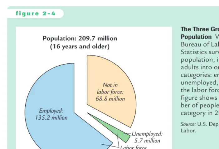
Today, economic data offer a systematic and objective source of information, and almost every day the newspaper has a story about some newly released statis-tic. Most of these statistics are produced by the government.Various government agencies survey households and firms to learn about their economic activity— how much they are earning, what they are buying, what prices they are charging, whether they have a job or are looking for work, and so on. From these surveys, various statistics are computed that summarize the state of the economy. Econo-mists use these statistics to study the economy; policymakers use them to moni-tor developments and formulate policies.
This chapter focuses on the three statistics that economists and policymakers use most often.Gross domestic product, or GDP, tells us the nation’s total income
| 15
2
The Data of Macroeconomics
C H A P T E R
It is a capital mistake to theorize before one has data. Insensibly one begins to twist facts to suit theories, instead of theories to fit facts.
and the total expenditure on its output of goods and services. The consumer price index, or CPI,measures the level of prices.The unemployment ratetells us the fraction of workers who are unemployed. In the following pages, we see how these statistics are computed and what they tell us about the economy.
2-1
Measuring the Value of Economic Activity:
Gross Domestic Product
Gross domestic product is often considered the best measure of how well the economy is performing.This statistic is computed every three months by the Bu-reau of Economic Analysis (a part of the U.S. Department of Commerce) from a large number of primary data sources.The goal of GDP is to summarize in a sin-gle number the dollar value of economic activity in a given period of time.
There are two ways to view this statistic. One way to view GDP is as the total income of everyone in the economy. Another way to view GDP is as the total expendi-ture on the economy’s output of goods and services. From either viewpoint, it is clear why GDP is a gauge of economic performance. GDP measures something peo-ple care about—their incomes. Similarly, an economy with a large output of goods and services can better satisfy the demands of households, firms, and the government.
How can GDP measure both the economy’s income and the expenditure on its output? The reason is that these two quantities are really the same: for the economy as a whole, income must equal expenditure.That fact, in turn, follows from an even more fundamental one: because every transaction has both a buyer and a seller, every dollar of expenditure by a buyer must become a dollar of in-come to a seller.When Joe paints Jane’s house for $1,000, that $1,000 is inin-come to Joe and expenditure by Jane. The transaction contributes $1,000 to GDP, re-gardless of whether we are adding up all income or adding up all expenditure.
To understand the meaning of GDP more fully, we turn to national income accounting, the accounting system used to measure GDP and many related statistics.
Income, Expenditure, and the Circular Flow
Imagine an economy that produces a single good, bread, from a single input, labor. Figure 2-1 illustrates all the economic transactions that occur between households and firms in this economy.
The inner loop in Figure 2-1 represents the flows of bread and labor. The households sell their labor to the firms.The firms use the labor of their workers to produce bread, which the firms in turn sell to the households. Hence, labor flows from households to firms, and bread flows from firms to households.
from these sales to pay the wages of their workers, and the remainder is the profit belonging to the owners of the firms (who themselves are part of the household sector). Hence, expenditure on bread flows from households to firms, and in-come in the form of wages and profit flows from firms to households.
GDP measures the flow of dollars in this economy. We can compute it in two ways. GDP is the total income from the production of bread, which equals the sum of wages and profit—the top half of the circular flow of dollars. GDP is also the total expenditure on purchases of bread—the bottom half of the circular flow of dollars.To compute GDP, we can look at either the flow of dollars from firms to households or the flow of dollars from households to firms.
These two ways of computing GDP must be equal because the expenditure of buyers on products is, by the rules of accounting, income to the sellers of those products. Every transaction that affects expenditure must affect income, and every transaction that affects income must affect expenditure. For example, suppose that a firm produces and sells one more loaf of bread to a household. Clearly this transaction raises total expenditure on bread, but it also has an equal effect on total income. If the firm produces the extra loaf without hiring any more labor (such as by making the production process more efficient), then profit increases. If the firm produces the extra loaf by hiring more labor, then wages increase. In both cases, expenditure and income increase equally.
f i g u r e 2 - 1
Income ($)
Labor
Goods (bread)
Expenditure ($)
Households Firms
Rules for Computing GDP
In an economy that produces only bread, we can compute GDP by adding up the total expenditure on bread. Real economies, however, include the produc-tion and sale of a vast number of goods and services.To compute GDP for such a complex economy, it will be helpful to have a more precise definition:gross
FYI
Many economic variables measure a quantity of something—a quantity of money, a quantity of goods, and so on. Economists distinguish be-tween two types of quantity variables: stocks and flows. A stockis a quantity measured at a given point in time, whereas a flowis a quantity mea-sured per unit of time.
The bathtub, shown in Figure 2-2, is the clas-sic example used to illustrate stocks and flows. The amount of water in the tub is a stock: it is the quantity of water in the tub at a given point in time. The amount of water coming out of the faucet is a flow: it is the quantity of water being added to the tub per unit of time. Note that we measure stocks and flows in different units. We say that the bathtub contains 50 gallonsof water, but that water is coming out of the faucet at 5 gallons per minute.
GDP is probably the most important flow variable in economics: it tells us how many dol-lars are flowing around the economy’s circular flow per unit of time. When you hear someone say that the U.S. GDP is $10 trillion, you should
Stocks and Flows
understand that this means that it is $10 trillion per year. (Equivalently, we could say that U.S. GDP is $317,000 per second.)
Stocks and flows are often related. In the bathtub example, these relationships are clear. The stock of water in the tub represents the accu-mulation of the flow out of the faucet, and the flow of water represents the change in the stock. When building theories to explain economic vari-ables, it is often useful to determine whether the variables are stocks or flows and whether any re-lationships link them.
Here are some examples of related stocks and flows that we study in future chapters:
➤ A person’s wealth is a stock; income and
ex-penditure are flows.
➤ The number of unemployed people is a stock;
the number of people losing their jobs is a flow.
➤ The amount of capital in the economy is a
stock; the amount of investment is a flow.
➤ The government debt is a stock; the
govern-ment budget deficit is a flow.
f i g u r e 2 - 2
domestic product (GDP) is the market value of all final goods and services produced within an economy in a given period of time.To see how this definition is applied, let’s dis-cuss some of the rules that economists follow in constructing this statistic.
Adding Apples and Oranges The U.S. economy produces many different goods and services—hamburgers, haircuts, cars, computers, and so on. GDP combines the value of these goods and services into a single measure.The diver-sity of products in the economy complicates the calculation of GDP because different products have different values.
Suppose, for example, that the economy produces four apples and three oranges. How do we compute GDP? We could simply add apples and oranges and conclude that GDP equals seven pieces of fruit. But this makes sense only if we thought ap-ples and oranges had equal value, which is generally not true. (This would be even clearer if the economy had produced four watermelons and three grapes.)
To compute the total value of different goods and services, the national in-come accounts use market prices because these prices reflect how much people are willing to pay for a good or service. Thus, if apples cost $0.50 each and or-anges cost $1.00 each, GDP would be
GDP equals $5.00—the value of all the apples, $2.00, plus the value of all the oranges, $3.00.
Used Goods When the Topps Company makes a package of baseball cards and sells it for 50 cents, that 50 cents is added to the nation’s GDP. But what about when a collector sells a rare Mickey Mantle card to another collector for $500? That $500 is not part of GDP. GDP measures the value of currently produced goods and services.The sale of the Mickey Mantle card reflects the transfer of an asset, not an addition to the economy’s income. Thus, the sale of used goods is not included as part of GDP.
The Treatment of Inventories Imagine that a bakery hires workers to produce more bread, pays their wages, and then fails to sell the additional bread. How does this transaction affect GDP?
The answer depends on what happens to the unsold bread. Let’s first suppose that the bread spoils. In this case, the firm has paid more in wages but has not re-ceived any additional revenue, so the firm’s profit is reduced by the amount that wages are increased. Total expenditure in the economy hasn’t changed because no one buys the bread. Total income hasn’t changed either—although more is distributed as wages and less as profit. Because the transaction affects neither ex-penditure nor income, it does not alter GDP.
Now suppose, instead, that the bread is put into inventory to be sold later. In this case, the transaction is treated differently. The owners of the firm are assumed to have “purchased’’ the bread for the firm’s inventory, and the firm’s profit is not
GDP = (Price of Apples ×Quantity of Apples) +(Price of Oranges ×Quantity of Oranges)
= ($0.50 ×4) +($1.00 ×3)
reduced by the additional wages it has paid. Because the higher wages raise total income, and greater spending on inventory raises total expenditure, the econ-omy’s GDP rises.
What happens later when the firm sells the bread out of inventory? This case is much like the sale of a used good.There is spending by bread consumers, but there is inventory disinvestment by the firm.This negative spending by the firm offsets the positive spending by consumers, so the sale out of inventory does not affect GDP.
The general rule is that when a firm increases its inventory of goods, this in-vestment in inventory is counted as expenditure by the firm owners.Thus, pro-duction for inventory increases GDP just as much as propro-duction for final sale. A sale out of inventory, however, is a combination of positive spending (the pur-chase) and negative spending (inventory disinvestment), so it does not influence GDP. This treatment of inventories ensures that GDP reflects the economy’s current production of goods and services.
Intermediate Goods and Value Added Many goods are produced in stages: raw materials are processed into intermediate goods by one firm and then sold to another firm for final processing. How should we treat such products when computing GDP? For example, suppose a cattle rancher sells one-quarter pound of meat to McDonald’s for $0.50, and then McDonald’s sells you a hamburger for $1.50. Should GDP include both the meat and the hamburger (a total of $2.00), or just the hamburger ($1.50)?
The answer is that GDP includes only the value of final goods.Thus, the ham-burger is included in GDP but the meat is not: GDP increases by $1.50, not by $2.00.The reason is that the value of intermediate goods is already included as part of the market price of the final goods in which they are used.To add the intermedi-ate goods to the final goods would be double counting—that is, the meat would be counted twice. Hence, GDP is the total value of final goods and services produced.
One way to compute the value of all final goods and services is to sum the value added at each stage of production.The value addedof a firm equals the value of the firm’s output less the value of the intermediate goods that the firm purchases. In the case of the hamburger, the value added of the rancher is $0.50 (assuming that the rancher bought no intermediate goods), and the value added of McDonald’s is $1.50 − $0.50, or $1.00. Total value added is $0.50 + $1.00, which equals $1.50. For the economy as a whole, the sum of all value added must equal the value of all final goods and services. Hence, GDP is also the total value added of all firms in the economy.
Housing Services and Other Imputations Although most goods and services are valued at their market prices when computing GDP, some are not sold in the marketplace and therefore do not have market prices. If GDP is to include the value of these goods and services, we must use an estimate of their value. Such an estimate is called an imputed value.
renters purchase.To take account of the housing services enjoyed by homeowners, GDP includes the “rent’’ that these homeowners “pay’’ to themselves. Of course, homeowners do not in fact pay themselves this rent. The Department of Com-merce estimates what the market rent for a house would be if it were rented and includes that imputed rent as part of GDP. This imputed rent is included both in the homeowner’s expenditure and in the homeowner’s income.
Imputations also arise in valuing government services. For example, police of-ficers, firefighters, and senators provide services to the public. Giving a value to these services is difficult because they are not sold in a marketplace and therefore do not have a market price.The national income accounts include these services in GDP by valuing them at their cost.That is, the wages of these public servants are used as a measure of the value of their output.
In many cases, an imputation is called for in principle but, to keep things sim-ple, is not made in practice. Because GDP includes the imputed rent on owner-occupied houses, one might expect it also to include the imputed rent on cars, lawn mowers, jewelry, and other durable goods owned by households. Yet the value of these rental services is left out of GDP. In addition, some of the output of the economy is produced and consumed at home and never enters the mar-ketplace. For example, meals cooked at home are similar to meals cooked at a restaurant, yet the value added in meals at home is left out of GDP.
Finally, no imputation is made for the value of goods and services sold in the
underground economy.The underground economy is the part of the economy that people hide from the government either because they wish to evade taxation or because the activity is illegal. Domestic workers paid “off the books” is one ex-ample.The illegal drug trade is another.
Because the imputations necessary for computing GDP are only approximate, and because the value of many goods and services is left out altogether, GDP is an imperfect measure of economic activity. These imperfections are most prob-lematic when comparing standards of living across countries.The size of the un-derground economy, for instance, varies from country to country.Yet as long as the magnitude of these imperfections remains fairly constant over time, GDP is useful for comparing economic activity from year to year.
Real GDP Versus Nominal GDP
Economists use the rules just described to compute GDP, which values the econ-omy’s total output of goods and services. But is GDP a good measure of eco-nomic well-being? Consider once again the economy that produces only apples and oranges. In this economy GDP is the sum of the value of all the apples pro-duced and the value of all the oranges propro-duced.That is,
Notice that GDP can increase either because prices rise or because quantities rise. It is easy to see that GDP computed this way is not a good gauge of eco-nomic well-being.That is, this measure does not accurately reflect how well the
economy can satisfy the demands of households, firms, and the government. If all prices doubled without any change in quantities, GDP would double.Yet it would be misleading to say that the economy’s ability to satisfy demands has doubled, because the quantity of every good produced remains the same. Econ-omists call the value of goods and services measured at current prices nominal GDP.
A better measure of economic well-being would tally the economy’s output of goods and services and would not be influenced by changes in prices. For this purpose, economists use real GDP, which is the value of goods and services measured using a constant set of prices.That is, real GDP shows what would have happened to expenditure on output if quantities had changed but prices had not. To see how real GDP is computed, imagine we wanted to compare output in 2002 and output in 2003 in our apple-and-orange economy. We could begin by choosing a set of prices, called base-year prices, such as the prices that prevailed in 2002. Goods and services are then added up using these base-year prices to value the different goods in both years. Real GDP for 2002 would be
Similarly, real GDP in 2003 would be
And real GDP in 2004 would be
Notice that 2002 prices are used to compute real GDP for all three years. Because the prices are held constant, real GDP varies from year to year only if the quanti-ties produced vary. Because a society’s ability to provide economic satisfaction for its members ultimately depends on the quantities of goods and services produced, real GDP provides a better measure of economic well-being than nominal GDP.
The GDP Deflator
From nominal GDP and real GDP we can compute a third statistic: the GDP de-flator. The GDP deflator, also called the implicit price deflator for GDP, is defined as the ratio of nominal GDP to real GDP:
GDP Deflator = .
The GDP deflator reflects what’s happening to the overall level of prices in the economy.
To better understand this, consider again an economy with only one good, bread. If Pis the price of bread and Qis the quantity sold, then nominal GDP is
Nominal GDP Real GDP
Real GDP =(2002 Price of Apples ×2004 Quantity of Apples) +(2002 Price of Oranges ×2004 Quantity of Oranges). Real GDP =(2002 Price of Apples ×2003 Quantity of Apples)
+(2002 Price of Oranges ×2003 Quantity of Oranges). Real GDP =(2002 Price of Apples ×2002 Quantity of Apples)
the total number of dollars spent on bread in that year,P×Q. Real GDP is the number of loaves of bread produced in that year times the price of bread in some base year,Pbase × Q. The GDP deflator is the price of bread in that year
relative to the price of bread in the base year,P/Pbase.
The definition of the GDP deflator allows us to separate nominal GDP into two parts: one part measures quantities (real GDP) and the other measures prices (the GDP deflator). That is,
Nominal GDP =Real GDP ×GDP Deflator.
Nominal GDP measures the current dollar value of the output of the economy. Real GDP measures output valued at constant prices. The GDP deflator measures the price of output relative to its price in the base year.We can also write this equation as
Real GDP = .
In this form, you can see how the deflator earns its name: it is used to deflate (that is, take inflation out of ) nominal GDP to yield real GDP.
Chain-Weighted Measures of Real GDP
We have been discussing real GDP as if the prices used to compute this measure never change from their base-year values. If this were truly the case, over time the prices would become more and more dated. For instance, the price of com-puters has fallen substantially in recent years, while the price of a year at college has risen.When valuing the production of computers and education, it would be misleading to use the prices that prevailed ten or twenty years ago.
To solve this problem, the Bureau of Economic Analysis used to update period-ically the prices used to compute real GDP. About every five years, a new base year was chosen. The prices were then held fixed and used to measure year-to-year changes in the production of goods and services until the base year was updated once again.
In 1995, the bureau announced a new policy for dealing with changes in the base year. In particular, it now emphasizes chain-weighted measures of real GDP. With these new measures, the base year changes continuously over time. In essence, average prices in 2001 and 2002 are used to measure real growth from 2001 to 2002; average prices in 2002 and 2003 are used to measure real growth from 2002 to 2003; and so on.These various year-to-year growth rates are then put together to form a “chain” that can be used to compare the output of goods and services between any two dates.
This new chain-weighted measure of real GDP is better than the more tradi-tional measure because it ensures that the prices used to compute real GDP are never far out of date. For most purposes, however, the differences are not impor-tant. It turns out that the two measures of real GDP are highly correlated with each other. The reason for this close association is that most relative prices change slowly over time. Thus, both measures of real GDP reflect the same thing: economy-wide changes in the production of goods and services.
The Components of Expenditure
Economists and policymakers care not only about the economy’s total output of goods and services but also about the allocation of this output among alternative uses. The national income accounts divide GDP into four broad categories of spending:
➤ Consumption (C) ➤ Investment (I)
➤ Government purchases (G) ➤ Net exports (NX).
Thus, letting Ystand for GDP,
Y=C+I+G+NX.
FYI
For manipulating many relationships in econom-ics, there is an arithmetic trick that is useful to know: the percentage change of a product of two vari-ables is approximately the sum of the percentage changes in each of the variables.
To see how this trick works, consider an exam-ple. Let Pdenote the GDP deflator and Ydenote real GDP. Nominal GDP is P×Y. The trick states
that
Percentage Change in (P×Y) ≈(Percentage Change in P)
+(Percentage Change in Y).
For instance, suppose that in one year, real GDP is 100 and the GDP deflator is 2; the next year, real GDP is 103 and the GDP deflator is 2.1. We can calculate that real GDP rose by 3 percent and that the GDP deflator rose by 5 percent. Nominal GDP rose from 200 the first year to 216.3 the second year, an increase of 8.15 per-cent. Notice that the growth in nominal GDP
Two Arithmetic Tricks for Working With
Percentage Changes
(8.15 percent) is approximately the sum of the growth in the GDP deflator (5 percent) and the growth in real GDP (3 percent).1
A second arithmetic trick follows as a corol-lary to the first: the percentage change of a ratio is ap-proximately the percentage change in the numerator minus the percentage change in the denominator. Again, consider an example. Let Y denote GDP and Ldenote the population, so that Y/Lis GDP per person. The second trick states
Percentage Change in (Y/L)
≈(Percentage Change in Y) −(Percentage Change in L).
For instance, suppose that in the first year, Yis 100,000 and Lis 100, so Y/Lis 1,000; in the sec-ond year, Y is 110,000 and L is 103, so Y/L is 1,068. Notice that the growth in GDP per person (6.8 percent) is approximately the growth in in-come (10 percent) minus the growth in popula-tion (3 percent).
1
Mathematical note:The proof that this trick works begins with the chain rule from calculus:
d(PY) =Y dP+P dY.
Now divide both sides of this equation by PYto obtain
d(PY)/(PY) =dP/P+dY/Y.
GDP is the sum of consumption, investment, government purchases, and net ex-ports. Each dollar of GDP falls into one of these categories.This equation is an
identity—an equation that must hold because of the way the variables are de-fined. It is called the national income accounts identity.
Consumptionconsists of the goods and services bought by households. It is divided into three subcategories: nondurable goods, durable goods, and services. Nondurable goods are goods that last only a short time, such as food and cloth-ing. Durable goods are goods that last a long time, such as cars and TVs. Services include the work done for consumers by individuals and firms, such as haircuts and doctor visits.
Investment consists of goods bought for future use. Investment is also di-vided into three subcategories: business fixed investment, residential fixed invest-ment, and inventory investment. Business fixed investment is the purchase of new plant and equipment by firms. Residential investment is the purchase of new housing by households and landlords. Inventory investment is the increase in firms’ inventories of goods (if inventories are falling, inventory investment is negative).
Government purchasesare the goods and services bought by federal, state, and local governments.This category includes such items as military equipment, highways, and the services that government workers provide. It does not include
FYI
Newcomers to macroeconomics are sometimes confused by how macroeconomists use familiar words in new and specific ways. One example is the term “investment.” The confusion arises be-cause what looks like investment for an individ-ual may not be investment for the economy as a whole. The general rule is that the economy’s in-vestment does not include purchases that merely reallocate existing assets among different individ-uals. Investment, as macroeconomists use the term, creates new capital.
Let’s consider some examples. Suppose we observe these two events:
➤ Smith buys for himself a 100-year-old
Victo-rian house.
➤ Jones builds for herself a brand-new
contem-porary house.
What is total investment here? Two houses, one house, or zero?
A macroeconomist seeing these two transac-tions counts only the Jones house as investment.
What Is Investment?
Smith’s transaction has not created new housing for the economy; it has merely reallocated exist-ing housexist-ing. Smith’s purchase is investment for Smith, but it is disinvestment for the person sell-ing the house. By contrast, Jones has added new housing to the economy; her new house is counted as investment.
Similarly, consider these two events:
➤ Gates buys $5 million in IBM stock from
Buf-fett on the New York Stock Exchange.
➤ General Motors sells $10 million in stock to
the public and uses the proceeds to build a new car factory.
transfer payments to individuals, such as Social Security and welfare. Because transfer payments reallocate existing income and are not made in exchange for goods and services, they are not part of GDP.
The last category,net exports, takes into account trade with other countries. Net exports are the value of goods and services exported to other countries minus the value of goods and services that foreigners provide us. Net exports represent the net expenditure from abroad on our goods and services, which provides income for domestic producers.
C A S E S T U D Y
GDP and Its Components
In 2000 the GDP of the United States totaled about $10 trillion.This number is so large that it is almost impossible to comprehend.We can make it easier to un-derstand by dividing it by the 2000 U.S. population of 275 million. In this way, we obtain GDP per person—the amount of expenditure for the average American— which equaled $36,174 in 2000.
Total Per Person
(billions of dollars) (dollars)
Gross Domestic Product 9,963.1 36,174
Consumption 6,757.3 24,534
Nondurable goods 2,010.0 7,298
Durable goods 820.3 2,978
Services 3,927.0 14,258
Investment 1,832.7 6,654
Nonresidential fixed investment 1,362.2 4,946 Residential fixed investment 416.0 1,510
Inventory investment 54.5 198
Government Purchases 1,743.7 6,331
Federal 595.2 2,161
Defense 377.0 1,369
Nondefense 218.2 792
State and local 1,148.6 4,170
Net Exports −370.7 −1,346
Exports 1,097.3 3,984
Imports 1,468.0 5,330
Source: U.S. Department of Commerce.
Other Measures of Income
The national income accounts include other measures of income that differ slightly in definition from GDP. It is important to be aware of the various mea-sures, because economists and the press often refer to them.
To see how the alternative measures of income relate to one another, we start with GDP and add or subtract various quantities. To obtain gross national product (GNP), we add receipts of factor income (wages, profit, and rent) from the rest of the world and subtract payments of factor income to the rest of the world:
GNP =GDP +Factor Payments From Abroad −Factor Payments to Abroad.
Whereas GDP measures the total income produced domestically, GNP measures the total income earned by nationals (residents of a nation). For instance, if a Japanese resident owns an apartment building in New York, the rental income he earns is part of U.S. GDP because it is earned in the United States. But because this rental income is a factor payment to abroad, it is not part of U.S. GNP. In the United States, factor payments from abroad and factor payments to abroad are similar in size—each representing about 3 percent of GDP—so GDP and GNP are quite close.
To obtain net national product (NNP), we subtract the depreciation of capital— the amount of the economy’s stock of plants, equipment, and residential struc-tures that wears out during the year:
NNP =GNP −Depreciation.
In the national income accounts, depreciation is called the consumption of fixed capital. It equals about 10 percent of GNP. Because the depreciation of capital is a cost of producing the output of the economy, subtracting depreciation shows the net result of economic activity.
The next adjustment in the national income accounts is for indirect business taxes, such as sales taxes.These taxes, which make up about 10 percent of NNP, place a wedge between the price that consumers pay for a good and the price How did this GDP get used? Table 2-1 shows that about two-thirds of it, or $24,534 per person, was spent on consumption. Investment was $6,654 per per-son. Government purchases were $6,331 per person, $1,369 of which was spent by the federal government on national defense.
that firms receive. Because firms never receive this tax wedge, it is not part of their income. Once we subtract indirect business taxes from NNP, we obtain a measure called national income:
National Income =NNP −Indirect Business Taxes.
National income measures how much everyone in the economy has earned. The national income accounts divide national income into five components, depending on the way the income is earned. The five categories, and the per-centage of national income paid in each category, are
➤ Compensation of employees(70%).The wages and fringe benefits earned by
workers.
➤ Proprietors’ income(9%).The income of noncorporate businesses, such as
small farms, mom-and-pop stores, and law partnerships.
➤ Rental income(2%).The income that landlords receive, including the
im-puted rent that homeowners “pay’’ to themselves, less expenses, such as de-preciation.
➤ Corporate profits(12%).The income of corporations after payments to their
workers and creditors.
➤ Net interest(7%).The interest domestic businesses pay minus the interest
they receive, plus interest earned from foreigners.
A series of adjustments takes us from national income to personal income, the amount of income that households and noncorporate businesses receive.Three of these adjustments are most important. First, we reduce national income by the amount that corporations earn but do not pay out, either because the corporations are retaining earnings or because they are paying taxes to the government.This ad-justment is made by subtracting corporate profits (which equals the sum of corpo-rate taxes, dividends, and retained earnings) and adding back dividends. Second, we increase national income by the net amount the government pays out in transfer payments.This adjustment equals government transfers to individuals minus social insurance contributions paid to the government.Third, we adjust national income to include the interest that households earn rather than the interest that businesses pay. This adjustment is made by adding personal interest income and subtracting net interest. (The difference between personal interest and net interest arises in part from the interest on the government debt.) Thus, personal income is
Personal Income =National Income −Corporate Profits
−Social Insurance Contributions
−Net Interest
+Dividends
+Government Transfers to Individuals
Next, if we subtract personal tax payments and certain nontax payments to the government (such as parking tickets), we obtain disposable personal income:
Disposable Personal Income
=Personal Income −Personal Tax and Nontax Payments.
We are interested in disposable personal income because it is the amount house-holds and noncorporate businesses have available to spend after satisfying their tax obligations to the government.
C A S E S T U D Y
The Seasonal Cycle and Seasonal Adjustment
Because real GDP and the other measures of income reflect how well the econ-omy is performing, economists are interested in studying the quarter-to-quarter fluctuations in these variables.Yet when we start to do so, one fact leaps out: all these measures of income exhibit a regular seasonal pattern. The output of the economy rises during the year, reaching a peak in the fourth quarter (October, November, and December), and then falling in the first quarter ( January, Febru-ary, and March) of the next year. These regular seasonal changes are substantial. From the fourth quarter to the first quarter, real GDP falls on average about 8 percent.2
It is not surprising that real GDP follows a seasonal cycle. Some of these changes are attributable to changes in our ability to produce: for example, build-ing homes is more difficult durbuild-ing the cold weather of winter than durbuild-ing other seasons. In addition, people have seasonal tastes: they have preferred times for such activities as vacations and holiday shopping.
When economists study fluctuations in real GDP and other economic vari-ables, they often want to eliminate the portion of fluctuations caused by pre-dictable seasonal changes. You will find that most of the economic statistics reported in the newspaper are seasonally adjusted.This means that the data have been adjusted to remove the regular seasonal fluctuations. (The precise statis-tical procedures used are too elaborate to bother with here, but in essence they involve subtracting those changes in income that are predictable simply from the change in season.) Therefore, when you observe a rise or fall in real GDP or any other data series, you must look beyond the seasonal cycle for the explanation.
2Robert B. Barsky and Jeffrey A. Miron, “The Seasonal Cycle and the Business Cycle,’’Journal of
2-2
Measuring the Cost of Living:
The Consumer Price Index
A dollar today doesn’t buy as much as it did 20 years ago. The cost of almost everything has gone up.This increase in the overall level of prices is called infla-tion, and it is one of the primary concerns of economists and policymakers. In later chapters we examine in detail the causes and effects of inflation. Here we discuss how economists measure changes in the cost of living.
The Price of a Basket of Goods
The most commonly used measure of the level of prices is the consumer price index (CPI).The Bureau of Labor Statistics, which is part of the U.S. Department of Labor, has the job of computing the CPI. It begins by collecting the prices of thousands of goods and services. Just as GDP turns the quantities of many goods and services into a single number measuring the value of production, the CPI turns the prices of many goods and services into a single index measuring the overall level of prices.
How should economists aggregate the many prices in the economy into a single index that reliably measures the price level? They could simply com-pute an average of all prices.Yet this approach would treat all goods and ser-vices equally. Because people buy more chicken than caviar, the price of chicken should have a greater weight in the CPI than the price of caviar. The Bureau of Labor Statistics weights different items by computing the price of a basket of goods and services purchased by a typical consumer.The CPI is the price of this basket of goods and services relative to the price of the same bas-ket in some base year.
For example, suppose that the typical consumer buys 5 apples and 2 oranges every month. Then the basket of goods consists of 5 apples and 2 oranges, and the CPI is
CPI = .
In this CPI, 2002 is the base year.The index tells us how much it costs now to buy 5 apples and 2 oranges relative to how much it cost to buy the same basket of fruit in 2002.
The consumer price index is the most closely watched index of prices, but it is not the only such index. Another is the producer price index, which mea-sures the price of a typical basket of goods bought by firms rather than con-sumers. In addition to these overall price indices, the Bureau of Labor Statistics computes price indices for specific types of goods, such as food, housing, and energy.
The CPI Versus the GDP Deflator
Earlier in this chapter we saw another measure of prices—the implicit price de-flator for GDP, which is the ratio of nominal GDP to real GDP. The GDP defla-tor and the CPI give somewhat different information about what’s happening to the overall level of prices in the economy. There are three key differences be-tween the two measures.
The first difference is that the GDP deflator measures the prices of all goods and services produced, whereas the CPI measures the prices of only the goods and services bought by consumers. Thus, an increase in the price of goods bought by firms or the government will show up in the GDP deflator but not in the CPI.
The second difference is that the GDP deflator includes only those goods produced domestically. Imported goods are not part of GDP and do not show up in the GDP deflator. Hence, an increase in the price of a Toyota made in Japan and sold in this country affects the CPI, because the Toyota is bought by con-sumers, but it does not affect the GDP deflator.
The third and most subtle difference results from the way the two measures aggregate the many prices in the economy. The CPI assigns fixed weights to the prices of different goods, whereas the GDP deflator assigns changing weights. In other words, the CPI is computed using a fixed basket of goods, whereas the GDP deflator allows the basket of goods to change over time as the composition of GDP changes. The following example shows how these approaches differ. Suppose that major frosts destroy the nation’s orange crop. The quantity of oranges produced falls to zero, and the price of the few or-anges that remain on grocers’ shelves is driven sky-high. Because oror-anges are no longer part of GDP, the increase in the price of oranges does not show up in the GDP deflator. But because the CPI is computed with a fixed basket of goods that includes oranges, the increase in the price of oranges causes a sub-stantial rise in the CPI.
Economists call a price index with a fixed basket of goods a Laspeyres index
and a price index with a changing basket a Paasche index. Economic theorists have studied the properties of these different types of price indices to determine which is a better measure of the cost of living. The answer, it turns out, is that neither is clearly superior.When prices of different goods are changing by differ-ent amounts, a Laspeyres (fixed basket) index tends to overstate the increase in the cost of living because it does not take into account that consumers have the opportunity to substitute less expensive goods for more expensive ones. By con-trast, a Paasche (changing basket) index tends to understate the increase in the cost of living. Although it accounts for the substitution of alternative goods, it does not reflect the reduction in consumers’ welfare that may result from such substitutions.
because the GDP deflator is a Paasche index, it understates the impact on con-sumers: the GDP deflator shows no rise in prices, yet surely the higher price of oranges makes consumers worse off.
Luckily, the difference between the GDP deflator and the CPI is usually not large in practice. Figure 2-3 shows the percentage change in the GDP deflator and the percentage change in the CPI for each year since 1948. Both measures usually tell the same story about how quickly prices are rising.
f i g u r e 2 - 3
16
14
12
10
8
6
4
2
0
−2
GDP deflator
Percentage change
1948 1953 1958 1963 1968 1973
Year
1978 1983 1988 1993 1998 2003
CPI
The GDP Deflator and the CPI This figure shows the percentage change in the GDP deflator and in the CPI for every year since 1948. Although these two measures of prices diverge at times, they usually tell the same story about how quickly prices are rising. Both the CPI and the GDP deflator show that prices rose slowly in most of the 1950s and 1960s, that they rose much more quickly in the 1970s, and that they rose slowly again in the 1980s and 1990s.
Source: U.S. Department of Commerce, U.S. Department of Labor.
C A S E S T U D Y
Does the CPI Overstate Inflation?
The consumer price index is a closely watched measure of inflation. Policymak-ers in the Federal Reserve monitor the CPI when choosing