on the Income Distribution of
Women with Children
Elizabeth O. Ananat
Guy Michaels
a b s t r a c t
Having a female first-born child significantly increases the probability that a woman’s first marriage breaks up. Using this exogenous variation, recent work finds that divorce has little effect on women’s mean household income. We further investigate the effect of divorce using Quantile Treatment Effect methodology and find that it increases women’s odds of having very high or very low income. In other words, while some women successfully compensate for lost spousal earnings through child support, welfare, combining households, and increasing labor supply, others are markedly unsuccessful. We conclude that by raising both poverty and inequality, divorce has important welfare consequences.
I. Introduction
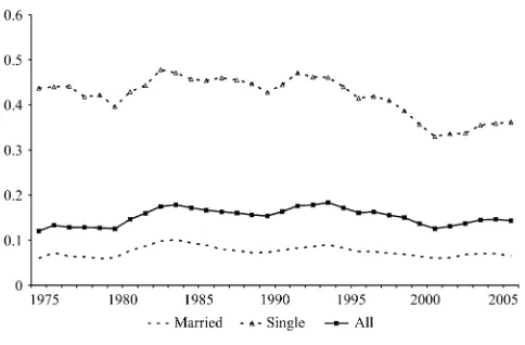
The poverty rate for single mothers fell substantially from 1974 to 2005. Over the same period, the poverty rate for married mothers remained virtually unchanged. Given these facts, one might assume that women with children are less likely to be poor than they were 30 years ago. But, in fact, the overall poverty rate for women with children rose over this period, from 0.120 to 0.143 (Figure 1). A clue to resolving this puzzle may be found in the fact that both divorce and single parent-hood have greatly increased over the past several decades throughout the developed
Elizabeth O. Ananat is an assistant professor of public policy at the Sanford Institute of Public Policy, Duke University, and a researcher at the National Bureau of Economic Research. Guy Michaels is a lecturer in the economics department and a researcher at the Centre for Economic Performance, London School of Economics, and a researcher at the Centre for Economic Policy Research. The authors thank Daron Acemoglu, Joshua Angrist, David Autor, and Jon Gruber. We also thank Alberto Abadie, Emek Basker, Joanna Lahey, Victor Lavy, Gerard Padro-i-Miquel, Ebonya Washington, Yoram Weiss, and participants at the labor economics and public economics workshops at MIT and the NBER Children’s meetings. Erin Harrison provided helpful research assistance. The data used in this article can be obtained beginning January 2009 through December 2012 from Guy Michaels, CEP, LSE, London WC2A 2AE, UK, g.michaels@lse.ac.uk
[Submitted September 2006; accepted July 2007]
ISSN 022-166X E-ISSN 1548-8004Ó2008 by the Board of Regents of the University of Wisconsin System
world. In the United States, the proportion of mothers who are single rose from about 16 percent in 1974 to more than 26 percent in 2005. Mechanically, it appears that in the absence of this trend, overall poverty rates would have decreased rather than in-creased. In this paper, we demonstrate that the relationship between a mother’s mar-ital status and her poverty status is not mere statistical artifact: We find that an exogenous increase in the probability that a woman’s first marriage breaks up leads to an increase in her chance of living in poverty, and that marital breakup exacerbates income inequality more broadly.
Political discussions have commonly assumed that marriage has causal economic effects on women and children. In particular, recent welfare legislation encourages marriage as a method of increasing income and reducing the need or eligibility for welfare. The federal government spends $150 million per year on the Healthy Mar-riage Promotion Program (DHHS 2007), part of its overall poverty-reduction plan; in addition, more than 40 state governments now make their own official efforts to sup-port marriage (Dion 2005).
Despite the assumptions made in popular debate, however, a causal relationship between marriage preservation and poverty reduction has not previously been dem-onstrated. Existing research has established the need for instrumental variable (IV) analysis in order to identify any effect of family status on women’s outcomes (Becker, Landes, and Michael 1977; Becker 1985; Angrist and Evans 1998; Gruber 2004). Recently, first-born child sex has emerged as an instrument for marital status, facilitating estimates of causality (Morgan and Pollard 2002, Lundberg and Rose 2003, Dahl and Moretti 2004). Using that instrument, Bedard and Deschenes (2005) conclude, ‘‘IV results cast doubt on the widely held view that divorce causes large declines in economic status for women’’ (p. 411). While it is true that the neg-ative correlation between mean income and divorce appears to be driven by selec-tion, we demonstrate in this paper that a conclusion based on the mean effect
Figure 1
of divorce is misleading. In fact, an examination of the impact of divorce on the en-tire income distribution supports the view that divorce greatly increases the odds of poverty.
This paper also uses the sex of the first-born child as an instrument for marital breakup and then conducts IV analysis to separate the causal effects of divorce from its well-known correlations. With data from the 1980 U.S. Census, we document that having a female first-born child slightly, but robustly, increases the probability that a woman’s first marriage breaks up. In our sample, the likelihood that a woman’s first marriage is broken is 0.63 percentage points higher if her first child is a girl, repre-senting a 3.7 percent increase from a base likelihood of 17.2 percentage points. A discussion of the mechanisms that drive this instrument, and detailed investigations into its validity and robustness, can be found in the working paper version of this paper (Ananat and Michaels 2007), in Bedard and Deschenes (2005) and in Dahl and Moretti (2004).
Unlike these previous papers, however, we use a Quantile Treatment Effect (QTE) estimation strategy (Abadie, Angrist, and Imbens 2002) that allows us to look at the impact of marital breakup throughout the income distribution. Using this technique, we find that marital breakup significantly affects the household income distribution. In particular, marital breakup dramatically increases the probability that a mother will end up with a very low income or a very high income.
It follows logically that divorce increases the probability of living in a household without other earners. In fact, we estimate that breakup of the first marriage signif-icantly increases the likelihood that a woman lives in a household with less than $5,000 of annual income from others—the likelihood rises from just over 5 percent for those whose first marriage is intact to nearly 50 percent for those whose first mar-riage breaks up. However, women can and do respond to income loss from divorce by combining with other households, through paths including remarriage or moving in with a roommate, sibling, or parents. Moreover, women further compensate through private (for example, alimony and child support) and public (for example, welfare) transfers, and by increasing their own labor supply. Because, further, di-vorce reduces family size as well as income, the net effect of the husband’s departure on the household’s income-to-needs ratio is ex ante ambiguous. In other words, it may be possible for a woman to entirely offset the loss of her husband’s income so that her material well-being is undiminished.
When examining the entire income distribution, however, we find that these responses, although substantial, are frequently insufficient to prevent poverty. While virtually none of the women influenced by our instrument who remain in their first marriage are in poverty, nearly a quarter of those who divorce are in poverty. In fact, IV results suggest that divorce causes an increase in poverty that is about as large as that suggested by the observed correlation between divorce and poverty.
who remain married. We conclude that breakup of the first marriage increases the variance of income, even though there is no significant effect on the mean. Because breakup of the first marriage leads some women to have higher incomes as well as leading more women to be poor, estimates that focus on the mean do not detect the dramatic effect that divorce has on the income distribution. That is, while divorce does not affect average income, it does exacerbate inequality and poverty. We view this result as part of a growing body of evidence on the importance of analyzing the effects of policy and social changes over the entire distribution of outcomes (Bitler, Gelbach, and Hoynes 2006; Neumark, Schweitzer, and Wascher, 2004; Blank and Schoeni 2003), rather then merely at the mean.
After discussing our findings, we consider the aggregate implications of the rela-tionship we identify between divorce, poverty, and inequality. In recent decades, mothers’ poverty rates have failed to decline as much as the overall poverty rate. At the same time, income inequality has increased. We argue that the increase in the proportion of broken first marriages in the United States can help account for both the stagnation in mothers’ poverty and the increase in income inequality.
II. Data and Instrument
We use data on women living with minor children from the 5 percent 1980 Census file (Ruggles et al. 2003), which allow us sufficient power to identify the effect of sex of the first-born child on marital breakup.1 We limit our sample to white women who are living with all of their children, whose eldest child is youn-ger than 17, who had their first birth after marriage, after age 18 and before age 45, and had a single first birth. These limitations are necessary in order to create a sam-ple for which measurement error in the sex of the observed first-born child has a clas-sical structure. Further discussion of the sample construction is contained in the Appendix.
First-born child sex has emerged in recent research as the preferred instrument for marital status in the United States for the era before prenatal ultrasound became com-mon (Bedard and Deschenes 2005; Dahl and Moretti 2004). Prior to routine ultra-sound, sex of the first child in the United States is believed to have served as a ‘‘coin flip’’ assigning couples with girls a higher divorce probability than couples with boys. This instrument passes an array of specification and falsification tests, and is quite robust (Ananat and Michaels 2007). Unfortunately, other potential instruments, such as state divorce law changes, do not pass such tests (Gruber 2004), which means that tests using overidentifying restrictions are not possible. Us-ing exact identification with eldest child’s sex as the sole instrument, we find that the probability that a woman’s first marriage is broken is 0.63 percentage points higher if her first child is a girl. Bedard and Deschenes (2005) use the same instrument and take a similar although not identical approach to sample limitation, getting estimates very close to ours. Dahl and Moretti (2004) show a variety of samples, the most sim-ilar of which gives first-stage estimates that are very close to ours.
III. Estimation Framework
In many applications of the Ordinary Least Squares (OLS) frame-work, researchers are interested in estimating the mean effect of a regressor (for ex-ample, the breakup of a woman’s first marriage) on various outcomes (such as measures of her income). The quantile regression (QR) model of Koenker and Bassett (1978) allows one to estimate the effect of a regressor not only on mean out-comes, but on the entire distribution of outcomes. Because we are interested in the distributional effects of divorce on income, this framework is useful for our purposes.
The endogeneity of marital breakup poses a challenge for interpreting the results of QR as the causal impact of divorce on the income distribution. But just as 2SLS can be used to overcome problems of omitted variables bias measurement error with OLS, so can the Quantile Treatment Effect (QTE) framework of Abadie, Angrist, and Imbens (2002) be used to overcome these problems in QR.
To apply the QTE model to our research question, we define our regressor of in-terest, D, as a dummy for the breakup of the first marriage. We consider a woman as having her first marriage intact if she reported both that she was ‘‘currently married with spouse present’’ and that she had been married exactly once. We consider a woman as having her first marriage broken if she: has been married multiple times, is married but currently not living with her husband, is currently separated from her husband, is currently divorced, or is currently widowed.2
Our main outcomes,Y, are total others’ income, defined as total household income less total own income; household income; and two measures of household income adjusted for household size. The change in others’ income measures the direct effect on a woman of losing her husband’s income (to the extent that the husband is not replaced by other wage earners). The change in total household income captures this direct effect but also includes the indirect effects of divorce on income: transfers from the ex-husband in the form of alimony and child support;3transfers from the state in the form of cash assistance; and income generated by changes in the woman’s own labor supply.4We use two methods to adjust household income for family com-position to capture the change in need that accompanies a change in household size. The first is household income as a percent of the federal poverty line; the second is household income divided by (number of adults + number of children0.7)0.7, a mea-sure used in Bedard and Deschenes (2005) and referred to as ‘‘normalized household income.’’
2. We have run the analysis with ever-divorced, rather than first marriage broken, as the explanatory vari-able: In this case, widows and those separated from or not living with their first husband are coded as 0 rather than 1. Our results are not sensitive to this difference in categorization.
3. The 1980 Census question reads: ‘‘Unemployment compensation, veterans’ payments, pensions, ali-mony or child support, or any other sources of income received regularly.Exclude lump-sum payments such as money from an inheritance or the sale of a home.’’
Our controls, denoted byX, are a vector of predetermined demographic variables, which include age, age squared, age at first birth, and an indicator for high-school drop-outs.5While our Ordinary Least Squares (OLS) and Quantile Regression (QR) esti-mates of the relationship between marital breakup and income may be sensitive to their inclusion, our IV specifications (both 2SLS and QTE) are robust to controls. We think of U as representing unobserved factors such as human capital, views on gen-der roles, and taste for nonmarket work relative to market work and leisure. Finally, our instrumental variable,Z, is an indicator for having a girl as one’s first born child.
We now consider two potential outcomes indexed againstD:Y1is the value a
wom-an’s outcome if her marriage breaks up, andY0is the outcome if the first marriage
remains intact. Similarly,D1tells us whether a woman’s first marriage is broken if
her eldest child is a girl, andD0tells us whether her first marriage is broken if her eldest
child is a boy. We are interested in the distribution of outcomes for women whose first marriage is broken and for women whose first marriage remains intact, and in the causal effect of divorce on the income distribution, which is the difference:Y1–Y0.
Abadie, Angrist, and Imbens (2002) provide assumptions under which we can es-timate a Quantile Treatment Effect (QTE) model:
(1) Independence: (Y1,Y0,D1,D0) is jointly independent ofZgivenX.
(2) Nontrivial assignment: 0 < P(Z¼1jX) < 1.
(3) First stage:E[D1jX]6¼ E[D0jX].
(4) Monotonicity:P(D1$D0jX)¼1.
(5) For eachu(0 <u< 1) there existauandbusuch thatQu(YjX,D,D1>D0)¼
auD+X’bu, whereQu(YjX,D,D1>D0) denote theu-quantile ofYgivenXandD
for compliers.
Under these assumptions, and additional regularity requirements (see Abadie, Angrist, and Imbens 2002) we can compute a consistent estimator of au and bu. The first four assumptions outlined above are very similar to the assumptions Angrist and Imbens (1994) use to derive the Local Average Treatment Effect (LATE) inter-pretation of 2SLS,6 and have been previously tested for the case of child sex as a predictor of divorce in Bedard and Deschenes (2005), Dahl and Moretti (2004), and the working paper version of this paper (Ananat and Michaels 2007). Finally, the fifth assumption requires that we can write a linear model of quantile regression, where our primary parameter of interest isau, which gives the difference in the con-ditionalu-quantiles ofY1andY0for compliers. In other words, just as IV can be used
5. Because we look only at women who gave birth to their first child at age 19 or later, we can reasonably assume that the decision on whether to graduate from high school is made prior to the realization of the sex of the first-born child.
to estimate the LATE of marital breakup on income for women whose first marriage is broken if and only if they have a girl (called ‘‘compliers’’ in the Angrist and Imbens literature), so can QTE estimate the effect of marital breakup on compliers’ income distribution.
IV. Results
The first column of Table 1 gives the estimated relationship between the sex of the first-born child and marital status for our sample. We find that having a girl increases the probability of breakup of the first marriage by about 0.63 percent; due to the large sample size, this effect is measured very precisely.7The effect of sex of the eldest child on the breakup of the first marriage is bigger than that on being currently divorced, which is 0.20 percent, because many of the women who divorced due to having a girl subsequently remarry (an endogenous response that is not
Table 1
Mean Regressions
First stage Second stage
Dependent variable Instrument: first child is a girl OLS 2SLS
First marriage is broken 0.0063 (0.0010) Currently divorced 0.0020
(0.0007)
OthersÕincome 29,241 21,041
(42.57) (5,178) Household income 25,577 6,548
(43,41) (5,570) Income/federal poverty line 259 27
(0.44) (53) Income/normalized
Household size
21,635 3,104
(18,34) (2,354)
Note: N¼619,499. The sample includes white women who are living with all of their children, whose eldest child is younger than 17, who had their first birth after marriage, after age 18 and before age 45, and whose first birth was a single birth. All the regressions include the following controls: age, age squared, age at first birth, and a dummy for high school dropouts. Poverty is calculated using 1980 Census codes that range in value from 1 to 501. Normalized income is windsorized at zero. Income is in 1980 dollars. 2SLS regressions use broken first marriage as the first-stage dependent variable. Robust standard errors are in parentheses.
properly part of our IV analysis). It is important to keep in mind that we are not es-timating the effect of being currently divorced or of residing in a mother-only house-hold on economic outcomes. Rather, we are estimating the effect of havingeverbeen divorced on current outcomes.
Cross-sectional (OLS) regressions of the relationship between marital breakup and various measures of income (shown in the second column of Table 1), which admit no causal interpretation, show that breakup of the first marriage is correlated with lower income. These relationships confirm the conventional view that women whose first mar-riages end are significantly worse off than women whose first marmar-riages remain intact. In the right-hand column, we replicate the results of Bedard and Deschenes (2005). Two-stage least squares estimates suggest that the mean causal effect of mar-ital breakup on material well-being is quite different from the population correlation. The two-stage estimate of the effect of divorce on others’ income is negative but in-significant and of much smaller magnitude than the OLS estimate. The two-stage es-timate of the effect of divorce on household income level, although not significantly different from zero, is positive and significantly different from the OLS estimate. The mean effects on adjusted household income and on income as a percent of poverty are both positive, but not precisely estimated. Bedard and Deschenes interpret these results as indicating that on average there is negative selection into divorce—women who would have had low income anyway are more likely to divorce, creating a neg-ative cross-sectional correlation between income and divorce—and that there is no significant causal effect of divorce on mean income.
Recent literature, however, has focused on and argued for the importance of exam-ining distributional effects rather than merely effects at the mean. Bitler, Gelbach, and Hoynes (2006), Neumark, Schweitzer, and Wascher (2004), Blank and Schoeni (2003) and others claim that analysis of the effects of policy and social changes should focus on effects throughout the distribution. Moreover, in the case of marital breakup, it seems highly plausible that there are important effects on the income dis-tribution that aren’t evident at the mean. After all, divorce—and the implied with-drawal of the husband’s income—represents a discrete fall in income. To the extent that women remarry, move in with parents or other relatives, or realize a high earning potential, they may end up as well or even better off financially than those who stay in their first marriage—resulting in little effect of divorce on the mean of the distribution. And those women who cannot find other sources of income could nonetheless experience large losses.
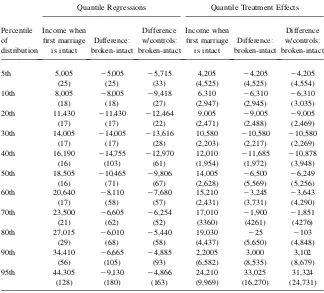
In Tables 2 and 3, the columns of results labeled ‘‘First marriage intact’’ report income at each decile of the distribution for those who remain married, estimated using the methods described above. Recall that in quantile treatment effects regres-sions, the income distributions are estimated for the specific group of women— ‘‘compliers’’—who divorce or stay married in response to the sex of the first-born child. The quantile regressions represent the income distributions for the population of women as a whole. The columns labeled ‘‘Difference in income: broken – intact’’ report the estimated difference in income at each decile of the distribution between those who have divorced and those who stay married, which is the coefficient on marital breakup.
associated with lower levels of income of others in the woman’s household through-out the distribution; the same is true for all deciles of total household income. In cross-section, women with broken first marriages have income distributions—both household and others’—that are first-order stochastically dominated by those of women whose first marriages remain intact. That is, divorce is correlated with a shift downward in income at every point in the income distribution.8
Table 2a
Cumulative Distribution of Other’s, Income by Marital Status
Quantile Regressions Quantile Treatment Effects
(25) (25) (33) (4,525) (4,525) (4,554) 10th 8,005 28,005 29,418 6,310 26,310 26,310
(18) (18) (27) (2,947) (2,945) (3,035) 20th 11,430 211,430 212,464 9,005 29,005 29,005
(17) (17) (22) (2,471) (2,488) (2,469) 30th 14,005 214,005 213,616 10,580 210,580 210,580
(17) (17) (28) (2,203) (2,217) (2,269) 40th 16,190 214,755 212,970 12,010 211,685 210,878
(16) (103) (61) (1,954) (1,972) (3,948) 50th 18,505 210,465 29,806 14,005 26,500 26,249
(16) (71) (67) (2,628) (5,569) (5,256) 60th 20,640 28,110 27,680 15,210 23,245 23,643
(17) (58) (57) (2,431) (3,731) (4,290) 70th 23,500 26,605 26,254 17,010 21,900 21,851
(21) (62) (52) (3360) (4261) (4276) 80th 27,015 26,010 25,440 19,030 225 2103
(29) (68) (58) (4,437) (5,650) (4,848) 90th 34,410 26,665 24,885 2,2005 3,000 3,102
(56) (105) (93) (6,582) (8,535) (8,679) 95th 44,305 29,130 24,866 24,210 33,025 31,324
(128) (180) (163) (9,969) (16,270) (24,731)
Note: N¼619,499. The sample includes white women who are living with all of their children, whose eldest child is under 17, who had their first birth after marriage, after age 18 and before age 45, and whose first birth was a single birth. All the regressions (except where indicated) include the following controls: age, age squared, age at first birth and a dummy for high school dropouts. Income is in 1980 dollars. QTE regressions use broken first marriage as the first-stage dependent variable. Robust standard errors in parentheses.
The quantile treatment effects (QTE) estimates, in the right panel of Table 2, give a more nuanced picture. We do in fact find a large effect of marital breakup on the probability of having very low income: Roughly 40 percent of women whose first marriage is broken have no household income due to any other household member. While legal transfers (which include child support and mean-tested transfers) reduce the number of compliers with no income, one in six of the divorced compliers have no unearned income even after accounting for transfers—compared to virtually none of the compliers who stay married. These effects on the bottom of the distribution are similar to the naı¨ve QR estimates.
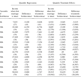
Table 2b
Cumulative Distribution of Household Income by Marital Status
Quantile Regressions Quantile Treatment Effects
5th 7,815 -5,100 -5,628 6,510 -5,045 -5,215 (27) (43) (41) (3,431) (3,849) (3,985) 10th 10,160 -6,150 -6,736 8,605 -5,100 -5,346 (19) -(33) (38) (2,779) (3,198) (3,035) 20th 14,285 -7,075 -7,441 11,185 -4,675 -5,003 (19) (41) (36) (2,683) (3,463) (3,239) 30th 17,205 -7,200 -7,512 13,340 -3,835 -4,484 (18) (36) (37) (2,593) (3,390) (3,201) 40th 19,910 -7,100 -7,154 15,165 -3,045 -3,635 (15) (43) (42) (2,345) (3,382) (3,616) 50th 22,010 -6,095 -6,363 17,015 -1,710 -2,243 (17) (49) (48) (2,768) (4,006) (4,027) 60th 24,770 -5,525 -5,338 19,005 -85 -435
(18) (54) (53) (3,107) (4,704) (4,393) 70th 27,810 -4,800 -4,258 20,795 2,080 1,691
(23) (61) (57) (3,412) (5,179) (5,104) 80th 31,950 -3,945 -3,163 23,020 5,195 4,769
(29) (72) (69) (4,567) (6,776) (6,367) 90th 40,005 -3,995 -1,954 26,435 13,690 12,793 (44) (112) (107) (7,091) (12,237) (12,998) 95th 50,010 -5,000 -1,747 29,515 32,635 31,185
(70) (182) (177) (10,942) (19,271) (26,205)
The analysis of household income, which adds in each woman’s own earnings, also shows a large effect of marital breakup on the bottom of the income distribution. Roughly one in six of those who experience marital breakup have less than $5,000 in household income, compared to virtually none of those who remain married.9
Interestingly, the QTE estimates also show that those who divorce due to the in-strument are more likely to have high levels of household income. These results
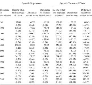
Table 3a
Cumulative Distribution of (Income/Federal Poverty Line) by Marital Status
Quantile Regressions Quantile Treatment Effects
(0.37) (0.64) (0.62) (39.51) (45.59) (46.73) 10th 138.00 278.00 278.74 128.00 274.00 275.26
(0.26) (0.46) (0.54) (41.32) (44.35) (40.77) 20th 194.00 290.00 281.18 171.00 290.00 285.76
(0.28) (0.58) (0.54) (37.21) (40.53) (42.56) 30th 234.00 285.00 279.01 207.00 295.00 286.39
(0.24) (0.59) (0.54) (35.10) (43.96) (44.16) 40th 270.00 282.00 275.23 238.00 289.00 278.13
(0.21) (0.60) (0.56) (34.97) (48.63) (47.30) 50th 304.00 276.00 271.20 262.00 267.00 257.04
(0.26) (0.69) (0.61) (33.64) (60.38) (56.59) 60th 341.00 270.00 264.88 284.00 225.00 220.80
(0.23) (0.66) (0.66) (31.09) (68.12) (65.92) 70th 386.00 266.00 256.31 307.00 27.00 27.41
(0.37) (0.82) (0.75) (30.75) (75.60) (70.02) 80th 446.00 258.00 241.12 329.00 97.00 93.94
(0.42) (1.08) (0.85) (35.54) (84.45) (81.63) 90th 501.00 0.00 25.01 356.00 145.00 136.86
(0.03) (0.09) (0.28) (44.43) (44.64) (57.67) 95th 501.00 0.00 0.00 375.00 126.00 125.00 (0.04) (0.09) (0.03) (61.03) (61.01) (65.19)
Note: N¼619,499. The sample includes white women who are living with all of their children, whose eldest child is under 17, who had their first birth after marriage, after age 18 and before age 45, and whose first birth was a single birth. All the regressions (except where indicated) include the following controls: age, age squared, age at first birth and a dummy for high school dropouts. Poverty is calculated using 1980 Cen-sus codes that range in value from 1 to 501. QTE regressions use broken first marriage as the first-stage dependent variable. Robust standard errors in parentheses.
diverge from naı¨ve QR estimates, suggesting that in the population at large negative selection into divorce swamps these effects and makes them undetectable. The top 20 percent of women whose first marriage breaks up because of a first-born girl have more income from others than do those who remain married. At the 95th percentile, women who divorce have more than twice as much income from others as do women who avoid divorce; the difference in the 95th percentile is statistically significant. Previous literature (Mueller and Pope 1980) finds that when divorced women remarry, their second husband is typically more educated and has a higher occupa-tional SES score. In addition, Bedard and Deschenes (2005) argue that many
Table 3b
Cumulative Distribution of (Income/Normalized HH Size) by Marital Status
Quantile Regressions Quantile Treatment Effects
(11) (21) (20) (1,355) (1,572) (1,610) 10th 4,348 22,223 22,247 4,266 22,607 22,608 60th 10,555 21,654 21,540 8,013 133 118
(8) (21) (20) (1,025) (1,762) (1,703) 70th 11,895 21,537 21,296 8,673 1,336 1,274
(10) (24) (23) (1,086) (2,168) (2,163) 80th 13,676 21,272 21,010 9,477 3,615 3,394
(13) (30) (29) (1,389) (3,150) (3,190) 90th 16,999 21,249 2653 10,538 8,830 8,195
(20) (47) (44) (2,060) (4,458) (5,365) 95th 21,234 21,694 2549 11,341 14,018 13,285
(35) (86) (68) (3,095) (4,964) (9,195)
divorced mothers coreside with their parents who, due to lifecycle effects, have higher incomes than their husbands did.10
When women’s own earnings are added in to reflect total household income, the magnitude of the effect of divorce on the top of the income distribution is even more striking, although less precise. Roughly 40 percent of women who divorce due to the instrument have higher household income than counterparts who remain married. This percentage may be higher because top-end variation in the rewards to women’s increased labor supply is added to top-end variation in the income of new household members.
As shown in Figure 2, the reversal in the sign of the income gap between those who divorce and those who do not occurs above the median of the distribution for all types of income, meaning that the typical family has less income when the first marriage breaks up. However, as is often the case with income distributions, average income among compliers is greater than median income (result available from the authors); as a result, the reversal occurs at (in the case of others’ income) or below (in the case of household income) themeanof the distribution. This statistical artifact explains why models that estimate effects at the mean, such as those in Bedard and Deschenes (2005), find little or positive effect of marital breakup on income.
The results discussed so far ignore one important aspect of divorce—namely, it reduces family size. Thus even if a woman loses income through divorce, she may not necessarily end up worse off if there are also fewer family members to support. On the other hand, if income gains at the top come heavily through combining house-holds, the effect may be neutralized or worse by increased household size. To esti-mate the effect of divorce on the ratio of income to needs, we divide each woman’s total household income by the federal poverty line (FPL) for a household of that size. Doing so also tells us about eligibility for programs such as Medicaid, SCHIP, free and reduced price lunch, and childcare subsidies, because eligibility cut-offs for these programs are based on FPL values such as 100 percent and 180 percent. We also use an alternative adjustment for family size used in Bedard and Deschenes (2005).
As shown in Table 3, we find that changes in family size do not fully offset the effect of marital breakup on household income. The naı¨ve QR estimates indicate that marital breakup decreases normalized household income at all levels. At the bottom of the income distribution, the QTE estimates are again comparable to naı¨ve QR esti-mates, showing that fewer than 5 percent of women still in their first marriage have household income below the poverty line, while nearly a quarter of those whose first marriage ended are below poverty. The bottom 40 percent of those who divorce due to the instrument have significantly lower income-to-needs ratios than their counter-parts who did not divorce.
Again, however, women whose first marriage ended are more likely to have very high income-to-needs ratios—higher than 400 percent of the FPL—than are com-pliers whose first marriage remains intact. The top ten percent of the comcom-pliers
Figure 2
who divorce have significantly higher normalized incomes than those who remain married. This reversal at the top is not picked up by naı¨ve QR estimates. The results are highly similar for the alternative normalization of household income.
V. Discussion
Our results confirm previous findings that negative selection into di-vorce accounts for the observed relationship between marital breakup and lower mean income. Yet marital breakup does have a significant causal effect on the distri-bution of income: it increases the percent of women at the bottom and top tails of the income distribution. On net, divorce increases poverty and inequality for women with children.
Our sample is not representative of all single mothers in the United States— although their first marriages are broken, many of the divorced compliers are not sin-gle when observed. In addition, the women we analyze were all married before their first child was born, so our results cannot be simply generalized to never-married mothers. Further, we are able to look only at white women; the effects of divorce may differ for women of other races. Nonetheless, examining this group of compliers has at least one significant advantage: The distribution of income for compliers who are still in their first marriage is somewhat, but not drastically, lower than the overall distribution of income in society. This characteristic suggests that the coeffi-cients we estimate reflect effects of divorce on women who are somewhat disadvan-taged and ‘‘at risk’’ yet not far outside the mainstream in terms of socioeconomic status.
Our results suggest that the destabilization of first marriages may have caused some of the stagnation in poverty rates of women with children over the last several decades. A back-of-the-envelope calculation suggests that the poverty rate among women with our sample characteristics was 14 percent (1.5 percentage points) higher in 1995 than it would have been had the share of broken first marriages remained at its 1980 level.11
Our results also suggest a relationship between the destabilization of first mar-riages and the widening of the income distribution. Previous literature has not em-phasized the relationship between divorce and inequality, although both have increased substantially over the past three decades. If early and sustained marriages act as a form of insurance against later shocks to either partner in earning capacity, then increased divorce in a sense weakens that insurance, and may be a factor in in-creasing household inequality. Much of the recent literature on the causes of income inequality has focused on wage inequality and the forces that may be affecting it,
such as technology (Acemoglu 2002); the decline of labor market institutions (DiNardo, Fortin, and Lemieux 1996); and the rise of international trade. Our find-ings suggest that the destabilization of first marriages may also be a contributing fac-tor to increasing income inequality.
Appendix 1
Data
The 5 percent 1980 Census data contain several measures that allow us to analyze a woman’s fertility history. These include the number of children ever born to a woman, the number of marriages, the quarter as well as year of first birth, and the quarter and year of first marriage. This information permits us to identify the sex of the first-born child for most women, although not for women whose eldest child has left the household.
A substantial drawback of using cross-sectional data is the fact that we can only observe the sex of the oldest child who resides with the mother, whereas ideally we would want to observe the sex of the first-born child. It is important that we create a sample of women for whom measurement error in the sex of the observed first-born child has a classical structure. To that end, we attempt to restrict the sample to those women observed with all their biological children. We do so in order to limit the risk that our results will be affected by differential attrition of boys and girls. In partic-ular, we are concerned that boys are differentially more likely to end up in the cus-tody of their fathers in the event of marital breakup. This pattern could lead to endogeneity of our instrument if the sample were left uncorrected. If, in the event of divorce, fathers keep the sons and mothers keep the daughters, there will be a spu-rious positive correlation in the overall sample between marital breakup and the el-destobservedchild being a girl.
To address this issue, we exclude from the sample any woman for whom the num-ber of children ever born does not equal the numnum-ber of children living with her. If a mother lives with stepchildren or adopted children in a number that exactly offsets the number of her own children that are not living with her, this rule will fail to ex-clude her. We therefore further minimize the possibility of including women who have nonbiological children ‘‘standing in’’ for biological children by including only women whose age at first birth is measured as between 19 and 44.
Limiting our sample to women who live with all their children reduces the risk that differential custody rates could bias our result, but it does not eliminate this risk al-together, because we could still be more likely to include divorced women with two girls than those with one boy and one girl or those with two boys. We have tested this hypothesis, however, and found that mothers living with all their children and moth-ers in the overall population are equally likely to be observed with a girl as the eldest child; this suggests that sex of the eldest child is not a major determinant of living with all of one’s children (results available from the authors).
selection into the first marriage (Lundberg and Rose 2003). To the extent that people could learn the sex of the child before it was born and thereby select into ‘‘shotgun marriages,’’ we may still have selection into first marriage. However, ultrasound technology was not yet widely used in 1980 (Campbell 2000), so this threat is not of particular concern. In addition, because we can only identify the beginning of the first marriage and not the end, we may include some women whose first child was born after the breakup of the first marriage. Although this would weaken the first stage of our estimation, it would not bias our results.
We look only at mothers whose eldest child is a minor, because those who still live with their adult children may be a select group. Further, because girls are differen-tially more likely to leave home early (at ages 17 and 18), we restrict the sample to mothers whose eldest child is younger than age 17. Fourth, we limit our sample to white women because black women are more likely to have girls, which necessi-tates analyzing them separately; unfortunately, the Census does not provide enough data for a strong first stage when restricting the sample to African-Americans only. Finally, we leave out any woman whose first child was a twin, both because different-sex twins would complicate our instrument and because twins increase the number of children a woman has.
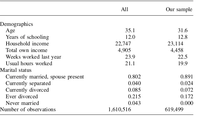
Table A1 shows summary statistics for our full sample relative to the overall ulation of women with minor children. Our sample is quite similar to the overall pop-ulation except in terms of age and marital status. The women in our sample are
Table 1A
Descriptive Statistics—Mothers with Minor Children Living at Home
All Our sample
Demographics
Age 35.1 31.6
Years of schooling 12.0 12.8
Household income 22,747 23,114
Total own income 4,905 4,458
Weeks worked last year 23.9 22.5
Usual hours worked 21.1 19.9
Marital status
Currently married, spouse present 0.802 0.891
Currently separated 0.040 0.024
Currently divorced 0.085 0.072
Ever divorced 0.215 0.172
Never married 0.043 0.000
Number of observations 1,610,516 619,499
younger than average, consistent with the requirement that a woman’s eldest child is younger than 17. The women in our sample are also slightly less likely to be di-vorced, both because they are younger and because we require that they have custody of all children. And of course, unlike the overall population, women in our sample cannot be never-married. On other characteristics, however, the two groups differ lit-tle: women in our sample have slightly more education and household income than the overall population and work and earn slightly less.
In summary, the limitations we place on the sample are designed to create a group of women for whom we can measure the sex of the first-born child with only clas-sical measurement error. These restrictions weaken the power of our first stage, but we believe this compromise is necessary in order to minimize concerns about endo-geneity of our instrument.
References
Acemoglu, Daron. 2002. ‘‘Technical Change, Inequality, and the Labor Market.’’Journal of Economic Literature40(1):7–72.
Abadie, Alberto, Joshua Angrist, and Imbens, Guido. 2002. ‘‘Instrumental Variables Estimates of the Effect of Subsidized Training on the Quantiles of Trainee Earnings.’’ Econometrica70(1):91–117.
Ananat, Elizabeth, and Guy Michaels. 2007. ‘‘The Effect of Marital Breakup on the Income Distribution of Women with Children.’’ Centre for Economic Policy Research: CEPR Discussion Paper No. 6228.
Angrist, Joshua, and William Evans. 1998. ‘‘Children and Their Parents’ Labor Supply: Evidence from Exogenous Variation in Family Size.’’American Economic Review 88(3):450–77.
Angrist, Joshua, and Guido Imbens. 1994. ‘‘Identification and Estimation of Local Average Treatment Effects.’’Econometrica62(2):467–76.
Becker, Gary. 1985. ‘‘Human Capital, Effort, and the Sexual Division of Labor.’’Journal of Labor Economics3(1):S33–58.
Becker, Gary, Elizabeth Landes, and Robert Michael. 1977. ‘‘An Economic Analysis of Marital Instability.’’Journal of Political Economy85(6):1141–87.
Bedard, Kelly, and Olivier Deschenes. 2005. ‘‘Sex Preferences, Marital Dissolution, and the Economic Status of Women.’’Journal of Human Resources40(2):411–34.
Bitler, Marianne, Jonah Gelbach, and Hilary Hoynes. 2006. ‘‘What Mean Impacts Miss: Distributional Effects of Welfare Reform Experiments.’’American Economic Review 96(4):988–1012.
Blank, Rebecca, and Robert Schoeni. 2003. ‘‘Changes in the Distribution of Children’s Family Income over the 1990’s.’’American Economic Review93(2):304–308.
Campbell, Stuart. 2000. ‘‘History of Ultrasound in Obstetrics and Gynecology.’’ presented at International Federation of Obstetrics and Gynecology, Washington, D.C. http:// www.obgyn.net/avtranscripts/FIGO_historycampbell.htm
Dahl, Gordon, and Enrico Moretti. 2004. ‘‘The Demand for Sons: Evidence from Divorce, Fertility, and Shotgun Marriage.’’ Cambridge, Mass.: National Bureau of Economic Research, Working Paper No. 10281.
Dion, Robin. 2005. ‘‘Healthy Marriage Programs: Learning What Works.’’The Future of Children15(2):139–56.
Gruber, Jonathan. 2004. ‘‘Is Making Divorce Easier Bad for Children? The Long Run Implications of Unilateral Divorce.’’Journal of Labor Economics22(4):799–833. Koenker, Roger, and Gilbert Bassett Jr. 1978. ‘‘Regression Quantiles.’’Econometrica
46(1):33–50.
Lundberg, Shelly, and Elaina Rose. 2003. ‘‘Child Gender and the Transition to Marriage.’’ Demography40(2):333–49.
Mueller, Charles, and Hallowell Pope. 1980. ‘‘Divorce and Female Remarriage Mobility: Data on Marriage Matches after Divorce for White Women.’’Social Forces58(3):726–38. Neumark, David, Mark Schweitzer, and William Wascher. 2005. ‘‘The Effects of Minimum
Wages on the Distribution of Family Incomes: A Nonparametric Analysis.’’Journal of Human Resources40(4):867–94.
Ruggles, Steven et al. 2003.Integrated Public Use Microdata Series: Version 3.0. Minneapolis: Historical Census Projects, University of Minnesota. http://www.ipums.org U.S. Bureau of the Census. 2004. ‘‘Marital Status of the Population 15 Years Old and Over,
by Sex and Race: 1950 to Present’’ http://www.census.gov/population/socdemo/hh-fam/ tabMS-1.xls