https://drive.google.com/file/d/0B z5oZTdyBW1NUkwVnJoMUVkU0k/view?pli=1

(1)

(2)

VARIABEL ACAK

Random Variables

(3)



Expektasi dari Variabel Acak Diskrit



Bernoulli Random Variable



The Binomial Random Variable



The Geometric Distribution



The Hypergeometric Distribution



The Poisson Distribution



Continuous Random Variables



Uniform Distribution



The Exponential Distribution

Random Variables

(4)

Setelah mempelajari bagian ini diharapkan dapat :



Membedakan variabel acak diskrit dan variabel acak kontinu



Menjelaskan bagaimana suatu var. acak membentuk distribusi

peluang



Menghitung statistik dari suatu variabel acak



Menghitung statistik dari suatu fungsi peubah acak



Menghitung statistik dari jumlah atau kombinasi linier suatu

variabel avak



Mengidentifikasi tipe distribusi dari variabel acak yang

diberikan

LEARNING OBJECTIVES

(5)

Berdasarkan kelahiran dari empat anak dengan jender yang

berbeda boy (B) dan girl (G). Akan terjadi

2*2*2*2=2

4

= 16

kemungkinan urutan yg berbeda

, atau ruang sampelnya adalah:

BBBB

BGBB

GBBB

GGBB

BBBG

BGBG

GBBG

GGBG

BBGB

BGGB

GBGB

GGGB

BBGG

BGGG

GBGG

GGGG

Jika Girl dan boy masing-2 adalah

equally likely

[P(G) = P(B) =

1/2], dan jender tiap anak adalah saling bebas maka

the

probability of each of these 16 possibilities is:

(1/2)(1/2)(1/2)(1/2) = 1/16.

3-1 Using Statistics

(6)

Banyaknya

girl (G)

dalam tiap set dari kelahiran kel dg empat anak:

BBBB (0)

BGBB (1)

GBBB (1)

GGBB (2)

BBBG (1)

BGBG (2)

GBBG (2)

GGBG (3)

BBGB (1)

BGGB (2)

GBGB (2)

GGGB (3)

BBGG (2)

BGGG (3)

GBGG (3)

GGGG (4)

Catatan:

•

Tiap hasil yang mungkin merupakan nilai numerik tunggal

,

•

Seluruh kejadian memiliki nilai numerik dan berbeda

•

Banyaknya girl adalah

random variable

:

A

random variable, X, adalah: suatu fungsi karena:

Random Variables

(7)

Random Variables (Continued)

BBBB BGBB GBBB BBBG BBGB GGBB GBBG BGBG BGGB GBGB BBGG BGGG GBGG GGGB GGBG GGGG

0

1

2

3

4

X

Sample Space

(8)

Misalkan variabel acak

X = 3

, artinya memiliki titik sampel yg mendukung

BGGG, GBGG, GGBG, atau GGGB ,

P(X = 3) = P(BGGG) + P(GBGG) + P(GGBG) + P(GGGB) = 4/16

Distribusi peluang dari suatu variabel acak adalah tabel yg berisikan seluruh

nilai yg mungkin dari variabel tsb yang berhubungan dengan nilai

peluangnya

.

x

P(x)

0

1/16

1

4/16

2

6/16

3

4/16

4

1/16

16/16=1

The Graphical Display for this

Probability Distribution

is shown on the next Slide.

The Graphical Display for this

Probability Distribution

(9)

Number of Girls, X

P ro b a b ili ty , P (X ) 4 3 2 1 0 0.4 0.3 0.2 0.1 0.0 1/ 16 4/ 16 6/ 16 4/ 16 1/ 16

Probability Distribution of the Number of Girls in Four Births

Number of Girls, X

P ro b a b ili ty , P (X ) 4 3 2 1 0 0.4 0.3 0.2 0.1 0.0 1/ 16 4/ 16 6/ 16 4/ 16 1/ 16

(10)

Consider the experiment of

tossing two six-sided dice

. There are

36 possible

outcomes

. Let the random variable

X represent the sum of the numbers on

the two dice

:

2 3 4 5 6 7

1,1 1,2 1,3 1,4 1,5 1,6 8 2,1 2,2 2,3 2,4 2,5 2,6 9 3,1 3,2 3,3 3,4 3,5 3,6 10 4,1 4,2 4,3 4,4 4,5 4,6 11 5,1 5,2 5,3 5,4 5,5 5,6 12 6,1 6,2 6,3 6,4 6,5 6,6

x P(x)*

2 1/36 3 2/36 4 3/36 5 4/36 6 5/36 7 6/36 8 5/36 9 4/36 10 3/36 11 2/36 12 1/36 1

x P(x)*

2 1/36 3 2/36 4 3/36 5 4/36 6 5/36 7 6/36 8 5/36 9 4/36 10 3/36 11 2/36 12 1/36 1 12 11 10 9 8 7 6 5 4 3 2 0.17 0.12 0.07 0.02 x p (x )

Probability Distribution of Sum of Two Dice

* Note that: P x( ) (6 (7 x) ) /2 36

Example 3-1

(11)

Suatu variabel acak

acak diskrit :



nilai-nilainya mempunyai peluang



mempunyai jeda antara nilai – nilainya



counts

Suatu variabel acak

acak diskrit :



nilai-nilainya mempunyai peluang



mempunyai jeda antara nilai – nilainya



counts

Suatu variabel

acak kontinu:



mempunyai nilai yang tidak berhingga



bergerak secara kontinu dari nilai ke nilai



nilai-2nya tidak terlihat langsung berhubungan dengan

peluangnya.



measures (e.g.: height, weight, speed, value, duration,

length)

Suatu variabel

acak kontinu

:



mempunyai nilai yang tidak berhingga



bergerak secara kontinu dari nilai ke nilai



nilai-2nya tidak terlihat langsung berhubungan dengan

peluangnya.



measures (e.g.: height, weight, speed, value, duration,

length)

Discrete and Continuous Random

Variables

(12)





1

0

1

0

1

.

for all values of x.

2.

Corollary:

all x

P x

P X

( )









Distribusi peluang dari variabel acak diskrit X

harus

memenuhi dua keadaan berikut :

Rules of Discrete Probability

Distributions

(13)

F x

P X x

P i

all i x

( )



(

 

)

( )





The

cumulative distribution function

,

F(x)

, of a discrete

random variable X is:

x P(x) F(x) 0 0.1 0.1 1 0.2 0.3 2 0.3 0.6 3 0.2 0.8 4 0.1 0.9 5 0.1 1.0

1.00

x P(x) F(x)

0 0.1 0.1 1 0.2 0.3 2 0.3 0.6 3 0.2 0.8 4 0.1 0.9 5 0.1 1.0

1.00 0 1 2 3 4 5

1 .0 0 .9 0 .8 0 .7 0 .6 0 .5 0 .4 0 .3 0 .2 0 .1 0 .0

x

F

(x

)

Cumulative Probability Distribution of the Number of Switches

Cumulative Distribution Function

(14)

x P(x) F(x) 0 0.1 0.1 1 0.2 0.3 2 0.3 0.6 3 0.2 0.8 4 0.1 0.9 5 0.1 1.0

1

x P(x) F(x)

0 0.1 0.1 1 0.2 0.3 2 0.3 0.6

3 0.2 0.8

4 0.1 0.9 5 0.1 1.0

1

The probability that

at most three switches

will occur:

Cumulative Distribution Function

Note:

(15)

x P(x) F(x)

0 0.1 0.1 1 0.2 0.3 2 0.3 0.6 3 0.2 0.8 4 0.1 0.9 5 0.1 1.0

1

The probability that

more than one switch

will occur:

Using Cumulative Probability

Distributions (Figure 3-8)

Note:

(16)

x P(x) F(x)

0 0.1 0.1 1 0.2 0.3 2 0.3 0.6 3 0.2 0.8 4 0.1 0.9 5 0.1 1.0

1

The probability that anywhere

from one to three

switches

will occur:

Using Cumulative Probability

Distributions (Figure 3-9)

Note:

(17)

Rata-rata dari suatu dist. Peluang adalah ukuran

pemusatan atau lokasi sebagai rata-rata dari

suatu dist.frek. Besarannya merupakan

rata-rata dibobot

, dengan nilai dari variabel acak

diboboti oleh peluangnya.

Rata-rata selalu diketahui sebagai

expected value

(or

expectation

) dari suatu

variabel acak .

Nilai Ekspektasi

dari variabel acak X

adalah sama dengan jumlah dari variabel

dikalikan dengan peluangnya

.





E X





xP x

all x

( )

x P(x) xP(x)

0 0.1 0.0

1 0.2 0.2

2 0.3 0.6

3 0.2 0.6

4 0.1 0.4

5 0.1 0.5

1.0 2.3 = E(X) = 

5 4 3 2 1 0

2.3

3-2 Expected Values of Discrete

Random Variables

(18)

Suppose you are playing a coin toss game in which you are

paid $1 if the coin turns up heads and you lose $1 when the

coin turns up tails. The expected value of this game is E(X) =

0. A game of chance with an expected payoff of 0 is called a

fair game

.

Suppose you are playing a coin toss game in which you are

paid $1 if the coin turns up heads and you lose $1 when the

coin turns up tails. The expected value of this game is

E(X) =

0.

A game of chance with an expected payoff of 0 is called a

fair game

.

x P(x) xP(x)

-1 0.5 -0.50 1 0.5 0.50 1.0 0.00 =

E(X)=

-1 1

0

A Fair Game

(19)

Number

of items, x P(x) xP(x) h(x) h(x)P(x)

5000 0.2 1000 2000 400

6000 0.3 1800 4000 1200

7000 0.2 1400 6000 1200

8000 0.2 1600 8000 1600

9000 0.1 900 10000 1000

1.0 6700 5400

Example 3-3

Example 3-3: Monthly sales of a certain product are believed to follow the given probability distribution. Suppose the company has a fixed monthly production cost of $8000 and that each item brings $2. Find the expected monthly profit h(X), from product sales.

E h X h x P x

all x

[ ( )]



( ) ( ) 5400

The

expected value of a

function

of a discrete random variable X is:

E h X

h x P x

all x

[ ( )]





( ) ( )

The expected value of a

linear function

of a random variable is:

E(aX+b)=aE(X)+b

In this case: E(2X-8000)=2E(X)-8000=(2)(6700)-8000=5400 In this case: E(2X-8000)=2E(X)-8000=(2)(6700)-8000=5400

Expected Value of a Function of a

Discrete Random Variables

(20)

The

variance

of a random variable is the expected

squared deviation from the mean:



2



2



2

2 2 2

2

    

  



  

 



V X E X x P x

E X E X x P x xP x

all x

all x all x

( ) [( ) ] ( ) ( )

( ) [ ( )] ( ) ( )

The

standard deviation

of a random variable is the

square root of its variance:

 

SD X

( )



V X

( )

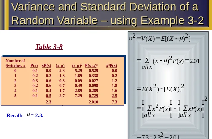
Variance and Standard Deviation of a

Random Variable

(21)

Number of

Switches, x P(x) xP(x) (x-) (x-)2 _P(x-_₎2 _x2_P(x)

0 0.1 0.0 -2.3 5.29 0.529 0.0 1 0.2 0.2 -1.3 1.69 0.338 0.2 2 0.3 0.6 -0.3 0.09 0.027 1.2 3 0.2 0.6 0.7 0.49 0.098 1.8 4 0.1 0.4 1.7 2.89 0.289 1.6 5 0.1 0.5 2.7 7.29 0.729 2.5

2.3 2.010 7.3

Number of

Switches, x P(x) xP(x) (x-) (x-)2 _P(x-_₎2 _x2_P(x)

0 0.1 0.0 -2.3 5.29 0.529 0.0 1 0.2 0.2 -1.3 1.69 0.338 0.2 2 0.3 0.6 -0.3 0.09 0.027 1.2 3 0.2 0.6 0.7 0.49 0.098 1.8 4 0.1 0.4 1.7 2.89 0.289 1.6 5 0.1 0.5 2.7 7.29 0.729 2.5 2.3 2.010 7.3





2

201

2

73 232 201















 



 













V X

E X

x

all x

P x

E X

x

all x

P x

all x

xP x

( )

[(

) ]

(

) ( )

.

(

) [ ( )]

( )

[image:21.720.9.720.20.485.2]

.

Table 3-8

Variance and Standard Deviation of a

Random Variable – using Example 3-2



(22)

The

variance

of a

linear function

of a random variable is:

V a X b a V X

(

 

)

2

( )



a

2



2

Number

of items, x P(x) xP(x) x2_P(x)

5000 0.2 1000 5000000 6000 0.3 1800 10800000 7000 0.2 1400 9800000 8000 0.2 1600 12800000 9000 0.1 900 8100000

1.0 6700 46500000

Example

3-3:

3:

    2 2 2 2 2 2 2 2 8000

46500000 6700 1610000 1610000 1268 86 2 8000 2

4 1610000 6440000 2 8000

2 2 1268 86 2537 72

                          



 V X

E X E X

x P x xP x

SD X

V X V X

SD x

all x all x

x x ( ) ( ) [ ( )] ( ) ( ) ( ) ( ) . ( ) ( ) ( ) ( )( ) ( ) ( )( . ) . ( )

Variance of a Linear Function of a

Random Variable

(23)

The

mean or expected value of the

sum

of random variables

is the sum of their means or expected values:



₍_{X Y}_ ₎



E X Y

(



)



E X

( )



E Y

( )





_X





_Y

For example: E(X) = $350 and E(Y) = $200

E(X+Y) = $350 + $200 = $550

The

variance of the

sum

of

mutually

independent

random

variables is the sum of their variances:



2



2



2

(X Y )



V X Y

(



)



V X

( )



V Y

( )



X



Y

if and only if X and Y are

independent.

For example: V(X) = 84 and V(Y) = 60

V(X+Y) = 144

Some Properties of Means and

Variances of Random Variables

(24)

The

variance of the

sum

of

k

mutually

independent

random

variables is the sum of their variances:

Some Properties of Means and

Variances of Random Variables

NOTE:

E

(

X

1



X

2



...



X

k

)



E

(

X

1

)



E

(

X

2

)



...



E

(

X

k

)

2

(

)

1

(

)

...

2

1

(

X

k

E

X

E

X

E

X

k

E







)

(

...

)

2

(

2

)

1

(

1

)

...

2

1

(

a

X

a

X

a

k

X

k

a

E

X

a

E

X

a

k

E

X

k

E







)



...



(

)

2

(

2

)

1

(

1

)

...

2

1

(

a

X

a

X

a

k

X

k

a

E

X

a

E

X

a

k

E

X

k

E







)

(

...

)

2

(

)

1

(

)

...

2

1

(

X

k

V

X

V

X

V

X

k

V







)

(

2

...

)

2

(

2

)

1

(

2

1

)

...

2

1

(

V

X

k

a

X

V

a

X

V

a

k

X

k

a

X

a

X

a

V







and

(25)

Chebyshev’s Theorem

applies to probability distributions just

as it applies to frequency distributions.

For a random variable X with mean



standard deviation



,

and for any number k > 1:

P X

k

(









)

 

1

₂

1

2

1

4

3

4

75%

1

3

1

9

8

9

89%

1

4

1

16

15

16

94%

2



 

 



 

 



 



At

least

Lie

within

Standard

deviations

of the mean

2

3

4

Chebyshev’s Theorem Applied to

Probability Distributions

(26)

Using the Template to Calculate

statistics of

(27)

Using the Template to Calculate Mean and Variance

for the Sum of Independent Random Variables

Output for Example 3-4

(28)

3-28

Dist.Peluang Var.Acak Diskrit

1. Dist Binom

2. Dist. Binom Negatif

3. Dist. Poisson

3. Dist Geometrik

4. Dist. Hipergeometrik

5. Dist.Multinom

(29)

•

If an experiment consists of a single trial and the outcome of the

trial can only be either a success

*

or a failure, then the trial is

called a

Bernoulli trial.

•

The number of success X in one Bernoulli trial, which can be 1 or

0, is a

Bernoulli random variable.

•

Note:

If p is the probability of success in a Bernoulli experiment,

the E(X) = p and V(X) = p(1 – p).

*

The terms

success

and

failure

are simply statistical terms, and do not have

positive or negative implications. In a production setting, finding a

defective product may be termed a “success,” although it is not a positive

result.

3-3 Bernoulli Random Variable

(30)

Consider a

Bernoulli Process

in which we have

a sequence of

n

identical

trials satisfying the following conditions:

1. Each trial has two possible outcomes, called

success

*and

failure

.

The two outcomes are

mutually exclusive

and

exhaustive

.

2. The

probability of success

, denoted by

p

, remains

constant

from trial

to trial. The

probability of failure

is denoted by

q

, where

q = 1-p

.

3. The

n

trials are

independent

. That is, the outcome of any trial does

not affect the outcomes of the other trials.

A random variable, X, that counts the number of successes in

n

Bernoulli

trials, where

p

is the probability of success* in any given trial, is said to

follow the

binomial probability distribution

with parameters

n

(number of trials) and

p

(probability of success). We call X the

binomial

random variable

.

* The terms success and failure are simply statistical terms, and do not have positive or negative implications. In a production setting, finding a defective product may be termed a “success,” although it is not a positive result.

3-4 The Binomial Random Variable

(31)

Suppose we toss a single fair and balanced coin five times in succession,

and let X represent the number of heads.

There are 25 _{= 32 possible sequences of H and T (S and F) in the sample space for this} experiment. Of these, there are 10 in which there are exactly 2 heads (X=2):

HHTTT HTHTH HTTHT HTTTH THHTT THTHT THTTH TTHHT TTHTH TTTHH

The probability of each of these 10 outcomes is p3_q3_{= (1/2)}3_(1/2)2_{=(1/32), so the} probability of 2 heads in 5 tosses of a fair and balanced coin is:

P(X = 2) = 10 * (1/32) = (10/32) = 0.3125

10 (1/32)

Number of outcomes with 2 heads

Probability of each outcome with 2 heads

Binomial Probabilities (Introduction)

(32)

10 (1/32) Number of outcomes

with 2 heads

Probability of each outcome with 2 heads

P(X=2) = 10 * (1/32) = (10/32) = .3125

Notice that this probability has two parts:

In general:

1. Theprobability of a given sequence

of x successes out of n trials with probability of success p and

probability of failure q is equal to:

p

x

q

(n-x)

nCx

n

x

n

x n x





 

!(



!

)!

2. The number of different sequences of n trials that result in exactly x successes is equal to the number of choices of x elements out of a total of n elements. This number is denoted:

Binomial Probabilities (continued)

(33)

Number of

successes, x Probability P(x)

0 1 2 3 n 1.00 n

n p q

n

n p q

n

n p q

n

n p q

n

n n n p q

n

n n n

! !( )! ! !( )! ! !( )! ! !( )! ! !( )! ( ) ( ) ( ) ( ) ( ) 0 0 1 1 2 2 3 3 0 0 1 1 2 2 3 3            

The binomial probability distribution:

where :

p is the probability of success in a single trial,

q = 1-p,

n is the number of trials, and

x is the number of successes.

P x

n

x

p q

n

x n x

p q

x n x x n x

( )

!

!(

)!

( ) ( )











The Binomial Probability Distribution

(34)

n=5

p

x 0.01 0.05 0.10 0.20 0.30 0.40 0.50 0.60 0.70 0.80 0.90 0.95 0.99 0 .951 .774 .590 .328 .168 .078 .031 .010 .002 .000 .000 .000 .000

1 .999 .977 .919 .737 .528 .337 .187 .087 .031 .007 .000 .000 .000 2 1.000 .999 .991 .942 .837 .683 .500 .317 .163 .058 .009 .001 .000 3 1.000 1.000 1.000 .993 .969 .913 .813 .663 .472 .263 .081 .023 .001 4 1.000 1.000 1.000 1.000 .998 .990 .969 .922 .832 .672 .410 .226 .049

h F(h) P(h)

0 0.031 0.031 1 0.187 0.156 2 0.500 0.313 3 0.813 0.313 4 0.969 0.156 5 1.000 0.031 1.000

Cumulative Binomial Probability Distribution and

Binomial Probability Distribution of H,the

Number of Heads Appearing in Five Tosses of

a Fair Coin

F x P X x P i

P F F

all i x

( ) ( ) ( )

( ) ( ) ( ) . .

.

  

    





P(X) = F(x) - F(x - 1)

For example:

3 3 2

813 500 313

Deriving Individual Probabilities from Cumulative Probabilities

The Cumulative Binomial Probability

Table (Table 1, Appendix C)

[image:34.720.32.705.29.473.2]

(35)

002

.

0

)

3

(

)

3

(

)

(

)

(

)

(















X

P

F

i

P

x

X

P

x

F

x i all

n=15

p

.50

.60

.70

0

.000

1

.000

2

.004

.000

3

.018

.002

.000

4

.059

.009

.001

...

60% of Brooke shares are owned by LeBow. A random sample

of 15 shares is chosen. What is the probability that

at most

three

of them will be found to be owned by LeBow?

60% of Brooke shares are owned by LeBow. A random sample

of 15 shares is chosen. What is the probability that

at most

three

of them will be found to be owned by LeBow?

Calculating Binomial Probabilities -

Example

(36)

Mean of a binomial distribution:

Variance of a binomial distribution:

Standard deviation of a binomial distribution:

= SD(X) = npq

2       

E X np

V X npq

( )

Mean of a binomial distribution:

Variance of a binomial distribution:

Standard deviation of a binomial distribution:

= SD(X) = npq

2       

E X np

V X npq

( ) ( )

118

.

1

25

.

1

)

(

25

.

1

)

5

)(.

5

)(.

5

(

)

(

5

.

2

)

5

)(.

5

(

)

(

2 : coin fair a of tosses five in heads of number the counts H if example, For



H

SD

H

V

H

E

H H H





Mean, Variance, and Standard

Deviation of the Binomial Distribution

(37)

Calculating Binomial Probabilities

using the Template

(38)

. . . . . . . . . . . . . . . . . . i 4 3 2 1 0 0.7 0.6 0.5 0.4 0.3 0.2 0.1 0.0 x P (x )

Binomial Probability: n=4 p=0.5

4 3 2 1 0 0.7 0.6 0.5 0.4 0.3 0.2 0.1 0.0 x P (x )

10 9 8 7 6 5 4 3 2 1 0 0 5 0 4 0 3 0 2 0 1 0 0 x P (x )

Binomial Probabil ty: n=10 p=0.5

20 19 18 17 16 15 14 13 12 11 10 9 8 7 6 5 4 3 2 1 0 0.2 0.1 0.0 x P (x )

Binomial distributions become more symmetric as n increases and as p 0.5.

p = 0.1 p = 0.3 p = 0.5

n = 4

n = 10

n = 20

Shape of the Binomial Distribution

(39)

The negative binomial distribution is useful for determining the probability of the number of trials made until the desired number of successes are achieved in a sequence of Bernoulli trials. It counts the number of trials X to achieve the number of successes s with p being the probability of success on each trial.

The negative binomial distribution is useful for determining the probability of the number of trials made until the desired number of successes are achieved in a sequence of Bernoulli trials. It counts the number of trials X to achieve the number of successes s with p being the probability of success on each trial.

) ( ) 1 ( 1 1 )

( ps p x s

s x x

X

P  

              : on Distributi Binomial Negative 2 ) 1 ( 2 : is variance The : is mean The p p s p s     

3-5 Negative Binomial Distribution

(40)

Negative Binomial Distribution - Example

Example:

Suppose that the probability of a manufacturing process

producing a defective item is 0.05. Suppose further that the quality of any one item is

independent of the quality of any other item produced. If a quality control officer selects items at random from the production line, what is the probability that the first

defective item is the eight item selected.

Here s = 1, x = 8, and p = 0.05. Thus,

0349

.

0

)

05

.

0

1

(

05

.

0

1

8

)

8

(

1 (8 1)













(41)

Calculating Negative Binomial

Probabilities using the Template

(42)

Geometric distribution:

where x = 1,2,3, . . . and and are the binomial parameters. The mean and variance of the geometric distribution are:

P x

pqx

p

q

p

( )







1

2

p q





Within the context of a binomial experiment, in which the outcome of each of

n

independent trials can be classified as a success (

S

) or a failure (

F

), the

geometric random variable

counts the

number of trials until the first success

..

Within the context of a binomial experiment, in which the outcome of each of

n

(.

)

1

(

P

) 1 4 ( ) 1 3 ( ) 1 2 ( ) 1 1 (



   

The Geometric Distribution - Example

(44)

Calculating Geometric Distribution

(45)

The hypergeometric probability distribution is useful for determining the

probability of a number of occurrences when sampling without replacement. It counts the number of successes (x) in n selections, without replacement, from a population of N elements, S of which are successes and (N-S) of which are failures.

The hypergeometric probability distribution is useful for determining the

probability of a number of occurrences when sampling without replacement. It counts the number of successes (x) in n selections, without replacement, from a population of N elements, S of which are successes and (N-S) of which are failures.

                                   





n

N

x

n

S

N

x

S

x

P

(

)

:

on

Distributi

tric

Hypergeome

The mean of the hypergeometric distribution is: where

The variance is:

      



np p S N N n N npq , 2 1

3-7 The Hypergeometric Distribution

(46)

Example:

Suppose that automobiles arrive at a dealership in lots of 10 and that for time and resource considerations, only 5 out of each 10 are inspected for safety. The 5 cars are randomly chosen from the 10 on the lot. If 2 out of the 10 cars on the lot are below standards for safety, what is the

probability that at least 1 out of the 5 cars to be inspected will be found not meeting safety standards?

Example:

Suppose that automobiles arrive at a dealership in lots of 10 and that for time and resource considerations, only 5 out of each 10 are inspected for safety. The 5 cars are randomly chosen from the 10 on the lot. If 2 out of the 10 cars on the lot are below standards for safety, what is the

probability that at least 1 out of the 5 cars to be inspected will be found not meeting safety standards?

 





 

  

 





 

  

 

P P ( ) ! ! ! ! ! ! ! ! ! . ( ) ! ! ! ! ! ! ! ! ! . 1 2 1 10 2 5 1 10 5 2 1 8 4 10 5 2 1 1 8 4 4 10 5 5 5 9 0 556 2 2 1 10 2 5 2 10 5 2 1 8 3 10 5 2 1 1 8 3 5 10 5 5 2

9 0 222

             



Thus, P(1) + P(2) =

0.556 + 0.222 = 0.778.

The Hypergeometric Distribution -

Example

(47)

Calculating Hypergeometric Distribution

(48)

The Poisson probability distribution is useful for determining the probability of a number of occurrences over a given period of time or within a given area or

volume. That is, the Poisson random variable counts occurrences over a

continuous interval of time or space. It can also be used to calculate approximate binomial probabilities when the probability of success is small (p 0.05) and the number of trials is large (n 20).

Poisson Distribution:

P x

e

x

( )

!







for x = 1,2,3,...

where  is the mean of the distribution (which also happens to be the variance) and

e is the base of natural logarithms (e=2.71828...).

3-8 The Poisson Distribution

(49)

Example 3-5:

Telephone manufacturers now offer 1000

different choices for a telephone (as

combinations of color, type, options, portability,

etc.). A company is opening a large regional

office, and each of its 200 managers is allowed to

order his or her own choice of a telephone.

Assuming independence of choices and that each

of the 1000 choices is equally likely, what is the

probability that a particular choice will be made

by none, one, two, or three of the managers?

n = 200



= np = (200)(0.001) = 0.2

p = 1/1000 = 0.001

Example 3-5:

Telephone manufacturers now offer 1000

different choices for a telephone (as

combinations of color, type, options, portability,

etc.). A company is opening a large regional

office, and each of its 200 managers is allowed to

order his or her own choice of a telephone.

Assuming independence of choices and that each

of the 1000 choices is equally likely, what is the

probability that a particular choice will be made

by none, one, two, or three of the managers?

n = 200



= np = (200)(0.001) = 0.2

p = 1/1000 = 0.001

P

e

P

e

P

e

P

e

( )

.

!

( )

.

!

( )

.

!

( )

.

!

. . . .

0

2

0

1

2

1

2

3

2

3

0 2 1 2 2 2 3 2



   

= 0.8187

= 0.1637

= 0.0164

= 0.0011

The Poisson Distribution - Example

(50)

Calculating Poisson Distribution

(51)

•

Poisson assumptions:



The probability that an event will occur in a short interval of time or space is proportional to the size of the interval.



In a very small interval, the probability that two events will occur is close to zero.



The probability that any number of events will occur in a given interval is independent of where the interval begins.



The probability of any number of events occurring over a given interval is independent of the number of events that occurred prior to the interval.

The Poisson Distribution (continued)

(52)

20 19 18 17 16 15 14 13 12 11 10 9 8 7 6 5 4 3 2 1 0 0.15 0.10 0.05 0.00 X P (x )

 = 10

10 9 8 7 6 5 4 3 2 1 0 0.2 0.1 0.0 X P (x )

 = 4

7 6 5 4 3 2 1 0 0.4 0.3 0.2 0.1 0.0 X P (x )

 = 1.5

4 3 2 1 0 0.4 0.3 0.2 0.1 0.0 X P (x )

 = 1.0

The Poisson Distribution (continued)

(53)

•

A discrete random variable:

 counts occurrences

 has a countable number of possible values

 has discrete jumps between successive values

 has measurable probability

associated with individual values

 probability is height

•

A continuous random variable:

 measures (e.g.: height, weight, speed,

value, duration, length)

 has an uncountably infinite number of

possible values

 moves continuously from value to

value

 has no measurable probability

associated with individual values

 probability is area

For example: Binomial n=3 p=.5 x P(x) 0 0.125 1 0.375 2 0.375 3 0.125 1.000 3 2 1 0 0.4 0.3 0.2 0.1 0.0 C1 P( x)

Binomial: n=3 p=.5

For example: In this case, the shaded area epresents the probability that the task takes between 2 and 3

minutes. 1 2 3 4 5 6

0.3 0.2 0.1 0.0 Minutes P( x)

Minutes to Complete Task

Discrete and Continuous Random

Variables - Revisited

(54)

6.5 6.0 5.5 5.0 4.5 4.0 3.5 3.0 2.5 2.0 1.5 1.0 0.15 0.10 0.05 0.00 Minutes P( x)

Minutes to Complete Task: By Half-Minutes

0.0. 0 1 2 3 4 5 6 7 Minutes

P(

x)

Minutes to Complete Task: Fourths of a Minute

Minutes

P(

x)

Minutes to Complete Task: Eighths of a Minute

0 1 2 3 4 5 6 7

The time it takes to complete a task can be subdivided into:

Half-Minute Intervals Quarter-Minute Intervals Eighth-Minute Intervals

Or even infinitesimally small intervals:

When a continuous random variable has been subdivided into infinitesimally small intervals, a measurable probability can only be associated with an interval of values, and the

probability is given by the area beneath the probability density function corresponding to that interval. In this example, the shaded area represents P(2 X 3).

When a continuous random variable has been subdivided into infinitesimally small intervals, a measurable probability can only be associated with an interval of values, and the

probability is given by the area beneath the probability density function corresponding to that interval. In this example, the shaded area represents P(2 X  ).

Minutes to Complete Task: Probability Density Function

7 6 5 4 3 2 1 0 Minutes f(z )

From a Discrete to a Continuous

Distribution

(55)

A continuous random variable is a random variable that can take on any value in an interval of numbers.

The probabilities associated with a continuous random variable X are determined by the

probability density function of the random variable. The function, denoted f(x), has the following properties.

1. f(x) 0 for all x.

2. The probability that X will be between two numbers a and b is equal to the area under f(x) between a and b.

3. The total area under the curve of f(x) is equal to 1.00.

The cumulative distribution function of a continuous random variable:

F(x) = P(X x) =Area under f(x) between the smallest possible value of X (often -)

and the point x.

A continuous random variable is a random variable that can take on any value in an interval of numbers.

The probabilities associated with a continuous random variable X are determined by the

probability density function of the random variable. The function, denoted f(x), has the following properties.

1. f(x) 0 for all x.

2. The probability that X will be between two numbers a and b is equal to the area under f(x) between a and b.

3. The total area under the curve of f(x) is equal to 1.00.

The cumulative distribution function of a continuous random variable:

F(x) = P(X x) =Area under f(x) between the smallest possible value of X (often -)

and the point x.

3-9 Continuous Random Variables

(56)

F(x)

f(x)

x

x 0

0

b a

F(b)

F(a) 1

b a

}

P(a X b) = Area under f(x) between a and b = F(b) - F(a)

P(a X b)=F(b) - F(a)

Probability Density Function and

(57)

3-10 Uniform Distribution

The uniform [a,b] density:

1/(a – b) for a X b f(x)=

0 otherwise

E(X) = (a + b)/2; V(X) = (b – a)2_/12

{

b b1

a

x

f(x

)

The entire area under f(x) = 1/(b – a) * (b – a) = 1.00

The area under f(x) from a1 to b1 =

P(a1Xb1)

= (b1 – a1)/(b – a)

a1

(58)

The uniform [0,5] density:

1/5 for 0 X

5

f(x)=

0 otherwise

E(X) = 2.5

{

6 5 4 3 2 1 0 -1 0.5

0.4

0.3

0.2

0.1

0.0 .

x

f(x

)

Uniform [0,5] Distribution

The entire area under f(x) = 1/5 * 5 = 1.00

The area under f(x) from 1 to 3 = P(1X3)

= (1/5)2 = 2/5

Uniform Distribution (continued)

(59)

Calculating Uniform Distribution

(60)

The exponential random variable measures the time between two occurrences that have a Poisson distribution.

Exponential distribution:

The density function is:

for

The mean and standard deviation are both equal to 1

The cumulative distribution function is:

for

f x e x

F x e x

x

x ( )

.

( ) .

  

  



 



0, 0

1 0

3 2

1 0

2

1

0

f(

x)

Exp onential Dis tributio n:  = 2

Time

3-11 Exponential Distribution

(61)

Example

The time a particular machine operates before breaking down (time between

breakdowns) is known to have an exponential distribution with parameter = 2. Time is

measured in hours. What is the probability that the machine will work continuously for at least one hour? What is the average time between breakdowns?

F x

e

P X

x

e

P X

e

x x

( )

(

)

(

)

.

( )( )

 











 



1

1353

2 1

 

E X

( )

  

1

.

2

5



Exponential Distribution - Example

(62)

Calculating Exponential Distribution