https://drive.google.com/file/d/0B z5oZTdyBW1NUkwVnJoMUVkU0k/view?pli=1

(1)

4-1

DISTRIBUSI VARIABEL ACAK

(2)

The Normal

(3)

4-3



Sifat-2 dari Dist.Normal



Dist. Normal Standard



Transformasi dari Variabel Acak Normal



Pendekatan Dist. Normal pada Dist.

Binomial

The Normal Distribution

(4)



Mengidentifikasi kapan variabel acak akan berdistribusi

normal



Mengetahui Kegunaan dari dist.normal



Menggunakan tabel distribusi normal untuk menghitung

peluang



Mentransformasi suatu distribusi normal ke dalam

distribusi normal standar.



Mengkonversi distribusi binomial ke dalam approximate

normal distribution

LEARNING OBJECTIVES

Setelah memepelajari bagian ini diharapkan dapat:

(5)

4-5

As

n

increases, the binomial distribution approaches a ...

n = 6

n = 10

n = 14

Normal Probability Density

Function:

6 5 4 3 2 1 0 0.3 0.2 0.1 0.0 x P (x )

Binomial Distribution: n=6, p=.5

10 9 8 7 6 5 4 3 2 1 0 0.3 0.2 0.1 0.0 x P (x )

14 13 12 11 10 9 8 7 6 5 4 3 2 1 0 0.3 0.2 0.1 0.0 x P (x )

5 0 -5 0.4 0.3 0.2 0.1 0.0 x f(x )

Normal Distribution:  = 0, 

(6)

The normal probability density function:

5 0

-5 0.4

0.3

0.2

0.1

0.0

x

f(x

)

Normal Distribution:  = 0, _{= 1}

Distribusi Peluang Normal

f x

e

x

e

( )

.

...

.

...





  

 



   

1

2

2 2

2 7182818

3 14159265









for

(7)

4-7

Sifat-2 dari Dist.Normal



Termasuk keluarga

Bell-shaped

dan Dist.

Symmetric,

karena d

istribusinya simetris, setengah disebelah kiri

dan setengah disebelah kanan sumbu rata-rata.



Variabel X disebut berdistribusi Normal Umum jika

mempunyai

mean

,



dan

variance

,









[

X~N(





)

]

(8)

•

Jika beberapa variabel acak yang saling bebas

berdist. Normal, maka jumlah dari variabel

tersebut akan berdistribusi normal juga.

•

Rata-rata dari jumlah variabel tersebut =

jumlah rata-ratanya.

(9)

4-9

Jika

X

1

, X

2

, …, X

n

adalah variabel acak normal, maka

Jumlah S juga akan berdist. Normal dengan:

•

E(S) = E(X

1

) + E(X

2

) + … + E(X

n

)

•

V(S) = V(X

1

) + V(X

2

) + … + V(X

n

)

(10)

Contoh -1 :

Misalkan

X

1

, X

2

, d

an

X

3

adalah

variabel acak yg saling

bebas yang mengikuti dist.normal dengan means dan

varians sbb:

Mean

Variance

X

1

10

1

X

2

20

2

X

3

30

3

Mis. S = X

1

+ X

2

+ X

3

. maka E(S) = 10 + 20 + 30 = 60 dan

V(S) = 1 + 2 + 3 = 6. Deviasi standar dari S adalah

= 2.45.

(11)

4-11

•

Jika

X

1

, X

2

, …, X

n

variabel acak normal, maka

variabel acak Q yaitu Q =

a

1

X

1

+ a

2

X

2

+ … +

a

n

X

n

+ b akan berdist. Normal juga dengan :

•

E(Q) = a

1

E(X

1

) + a

2

E(X

2

) + … + a

n

E(X

n

) + b

•

V(Q) = a

12

V(X

1

) + a

22

V(X

2

) + … + a

n2

V(X

n

)

•

Catatan:

Tidak berlaku bagi simpangan

(12)

Contoh-2 :

Misal

X

1

, X

2

, X

3

d

an

X

4

adalah variabel acak yg berdist. Normaln

dengan

means dan varians di bawah ini. Tentukan mean dan

varians dari Q =

X

1

- 2X

2

+ 3X

2

- 4X

4

+ 5

Mean

Variance

X

1

12

4

X

2

-5

2

X

3

8

5

X

4

10

1

E(Q) = 12 – 2(-5) + 3(8) – 4(10) + 5 = 11

V(Q) = 4 + (-2)

2

(2) + 3

2

(5) + (-4)

2

(1) = 73

(13)

4-13

Computing the Mean, Variance and Standard

Deviation for the Sum of Independent Random

Variables Using the Template

(14)

Seluruh fungsi densitas normal masing-2 dengan mean dan varians berbeda

Z~N(0,1)

5 0

-5 0.4

0.3

0.2

0.1

0.0

z

f(z

)

Normal Distribution:



=0,



=1

W~N(40,1)

X~N(30,25)

45 40

35 0.4

0.3

0.2

0.1

0.0

w

f(w

)



=40,



=1

60 50 40 30 20 10 0 0.2

0.1

0.0

x

f(x

)



=30,



=5

Y~N(50,9)

65 55

45 35

0.2

0.1

0.0

y

f(y

)

Normal Distribution:



=50,



=3

50

Consider:

P(39



W



41)

P(25



X



35)

P(47



Y



53)

P(-1



Z



1)

Peluang masing-2

merupakan daerah di

bawah kurva fungsi

densitas.

(15)

4-15

4-3 Computing Normal Probabilities

(16)

Z adalah

standard normal random variable

, dengan mean



= 0

dan deviasi standar



= 1

:

Z~N(0,1

2

)

.

5 4

3 2

1 0

- 1 - 2

- 3 - 4

- 5 0 . 4

0 . 3

0 . 2

0 . 1

0 . 0

Z

f(

z)

Standard Normal Distribution



= 0



{

=1

Dist. Normal Standar

(17)

4-17

z .00 .01 .02 .03 .04 .05 .06 .07 .08 .09

0.0 0.0000 0.0040 0.0080 0.0120 0.0160 0.0199 0.0239 0.0279 0.0319 0.0359 0.1 0.0398 0.0438 0.0478 0.0517 0.0557 0.0596 0.0636 0.0675 0.0714 0.0753 0.2 0.0793 0.0832 0.0871 0.0910 0.0948 0.0987 0.1026 0.1064 0.1103 0.1141 0.3 0.1179 0.1217 0.1255 0.1293 0.1331 0.1368 0.1406 0.1443 0.1480 0.1517 0.4 0.1554 0.1591 0.1628 0.1664 0.1700 0.1736 0.1772 0.1808 0.1844 0.1879 0.5 0.1915 0.1950 0.1985 0.2019 0.2054 0.2088 0.2123 0.2157 0.2190 0.2224 0.6 0.2257 0.2291 0.2324 0.2357 0.2389 0.2422 0.2454 0.2486 0.2517 0.2549 0.7 0.2580 0.2611 0.2642 0.2673 0.2704 0.2734 0.2764 0.2794 0.2823 0.2852 0.8 0.2881 0.2910 0.2939 0.2967 0.2995 0.3023 0.3051 0.3078 0.3106 0.3133 0.9 0.3159 0.3186 0.3212 0.3238 0.3264 0.3289 0.3315 0.3340 0.3365 0.3389 1.0 0.3413 0.3438 0.3461 0.3485 0.3508 0.3531 0.3554 0.3577 0.3599 0.3621 1.1 0.3643 0.3665 0.3686 0.3708 0.3729 0.3749 0.3770 0.3790 0.3810 0.3830 1.2 0.3849 0.3869 0.3888 0.3907 0.3925 0.3944 0.3962 0.3980 0.3997 0.4015 1.3 0.4032 0.4049 0.4066 0.4082 0.4099 0.4115 0.4131 0.4147 0.4162 0.4177 1.4 0.4192 0.4207 0.4222 0.4236 0.4251 0.4265 0.4279 0.4292 0.4306 0.4319

1.5 0.4332 0.4345 0.4357 0.4370 0.4382 0.4394 0.4406 0.4418 0.4429 0.4441 1.6 0.4452 0.4463 0.4474 0.4484 0.4495 0.4505 0.4515 0.4525 0.4535 0.4545 1.7 0.4554 0.4564 0.4573 0.4582 0.4591 0.4599 0.4608 0.4616 0.4625 0.4633 1.8 0.4641 0.4649 0.4656 0.4664 0.4671 0.4678 0.4686 0.4693 0.4699 0.4706 1.9 0.4713 0.4719 0.4726 0.4732 0.4738 0.4744 0.4750 0.4756 0.4761 0.4767 2.0 0.4772 0.4778 0.4783 0.4788 0.4793 0.4798 0.4803 0.4808 0.4812 0.4817 2.1 0.4821 0.4826 0.4830 0.4834 0.4838 0.4842 0.4846 0.4850 0.4854 0.4857 2.2 0.4861 0.4864 0.4868 0.4871 0.4875 0.4878 0.4881 0.4884 0.4887 0.4890 2.3 0.4893 0.4896 0.4898 0.4901 0.4904 0.4906 0.4909 0.4911 0.4913 0.4916 2.4 0.4918 0.4920 0.4922 0.4925 0.4927 0.4929 0.4931 0.4932 0.4934 0.4936 2.5 0.4938 0.4940 0.4941 0.4943 0.4945 0.4946 0.4948 0.4949 0.4951 0.4952 2.6 0.4953 0.4955 0.4956 0.4957 0.4959 0.4960 0.4961 0.4962 0.4963 0.4964 2.7 0.4965 0.4966 0.4967 0.4968 0.4969 0.4970 0.4971 0.4972 0.4973 0.4974 2.8 0.4974 0.4975 0.4976 0.4977 0.4977 0.4978 0.4979 0.4979 0.4980 0.4981 2.9 0.4981 0.4982 0.4982 0.4983 0.4984 0.4984 0.4985 0.4985 0.4986 0.4986 3.0 0.4987 0.4987 0.4987 0.4988 0.4988 0.4989 0.4989 0.4989 0.4990 0.4990

5 4 3 2 1 0 -1 -2 -3 -4 -5 0.4

0.3

0.2

0.1

0.0

Z

f(z

)

Standard Normal Distribution

1.56

{

Standard Normal Probabilities

Look in row labeled

1.5

and column labeled

.06

to

find

P(0



z



1.56) =

0.4406

Finding Probabilities of the Standard

(18)

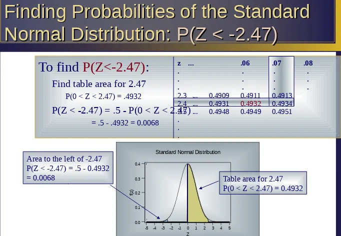
P(Z < -2.47)

To find

P(Z<-2.47)

:

Find table area for 2.47

P(0 < Z < 2.47) = .4932

P(Z < -2.47) = .5 - P(0 < Z < 2.47)

= .5 - .4932 = 0.0068

5 4 3 2 1 0 -1 -2 -3 -4 -5 0.4

0.3

0.2

0.1

0.0

Z

f(

z)

[image:18.720.38.720.24.496.2]

Table area for 2.47

P(0 < Z < 2.47) = 0.4932

Area to the left of -2.47

P(Z < -2.47) = .5 - 0.4932

= 0.0068

z ...

.06

.07

.08

.

2.3 ...

0.4909

0.4911

0.4913

2.4 ...

0.4931

0.4932

0.4934

2.5 ...

0.4948

0.4949

0.4951

.

(19)

4-19

Finding Probabilities of the Standard

P(1< Z < 2)

z .00 ...

. . . . . .

0.9 0.3159 ... 1.0 0.3413 ... 1.1 0.3643 ... . .

. . . .

1.9 0.4713 ... 2.0 0.4772 ... 2.1 0.4821 ... . .

. . . .

To find

P(1



Z



2)

:

1. Find table area for 2.00

F(2) = P(Z



2.00) = .5 + .4772 =.9772

2. Find table area for 1.00

F(1) = P(Z



1.00) = .5 + .3413 = .8413

3. P(1



Z



2.00) = P(Z



2.00) - P(Z



1.00)

= .9772 - .8413 =

0.1359

5 4 3 2 1 0 -1 -2 -3 -4 -5 0.4

0.3

0.2

0.1

0.0

Z

f(z

)

Area between 1 and 2

(20)

Random Variable:

P(0 < Z < z) = 0.40

To find

z

such that

P(0



Z



z) = .40:

1. Find a probability as close as

possible to .40 in the table of

standard normal probabilities.

2. Then determine the value of

z

from the corresponding row

and column.

P(0



Z



1.28

)



.40

Also, since

P(Z



0) = .50

P(Z



1.28

)



.90

-5 -4 -3 -2 -1 0 1 2 3 4 5

0.4

0.3

0.2

0.1

0.0

Z

f(

z)

Area = .40 (.3997)

Z = 1.28

Area to the left of 0 = .50

P(z



0) = .50

z .00 .01 .02 .03 .04 .05 .06 .07 .08 .09

(21)

4-21

z .04 .05 .06 .07 .08 .09

. . . . . . . . . . . . . . . 2.4 ... 0.4927 0.4929 0.4931 0.4932 0.4934 0.4936 2.5 ... 0.4945 0.4946 0.4948 0.4949 0.4951 0.4952 2.6 ... 0.4959 0.4960 0.4961 0.4962 0.4963 0.4964 . . . . . . . . . . . .

To have

.99

in the center of the distribution, there

should be

(1/2)(1-.99) = (1/2)(.01) = .005

in each

tail of the distribution, and

(1/2)(.99) = .495

in

each half of the

.99

interval. That is:

P(0



Z



z

.005

) = .495

Look to the table of standard normal probabilities

to find that:





 

z

.005

 

 

z

.005



P(-.2575



Z



) = .99

To have

.99

in the center of the distribution, there

should be

(1/2)(1-.99) = (1/2)(.01) = .005

in each

tail of the distribution, and

(1/2)(.99) = .495

in

each half of the

.99

interval. That is:

P(0



Z



z

.005

) = .495

Look to the table of standard normal probabilities

to find that:

   

z

.005

  

z

.005



P(-.2575



Z



) = .99

5 4 3 2 1 0 -1 -2 -3 -4 -5 0.4

0.3

0.2

0.1

0.0

Z

f(z

)

-z

_.005

z

_.005

Area in right tail = .005

Area in left tail = .005

Area in center right = .495

Area in center left = .495

2.575

-2.575

Total area in center = .99

(22)

The area within

k



of the mean is the same for all normal random variables. So an

area under any normal distribution is equivalent to an area under the standard normal. In

this example: P(40



X







P(-1



Z

  







since

 



and



The area within

k



of the mean is the same for all normal random variables

.

So an

area under any normal distribution is equivalent to an area under the standard normal

. In

this example: P(40



X

  

P(-1



Z



since



and



100 90 80 70 60 50 40 30 20 10 0 0.07 0.06 0.05 0.04 0.03 0.02 0.01 0.00 X f(x )



=50,



=10



{

=10

5 4 3 2 1 0 -1 -2 -3 -4 -5 0.4 0.3 0.2 0.1 0.0 Z f(z )

1.0

{

Transformation

(2) Division by



_x

)

The transformation of

X

to

Z

:

X

to

Z

:

The inverse transformation of

Z

to

X

:

Z

to

X

:

Random Variables

(1) Subtraction: (X -



_x

)

Z

X

x









(23)

4-23

Example 4-9

X~N(160,30

2

)

Example 4-9

X~N(160,30

2

)

Example 4-10

X~N(127,22

2

)

Example 4-10

X~N(127,22

2

)

Using the Normal Transformation





P

X

P

X

P

Z

P

Z

(

)

.

100

180

100

180

100 160

30

180 160

30

2

6667

0 4772 0 2475

0 7247



































































P X

P

X

P Z

(

)

.





























150

150 127

22

1 045

0 5 0 3520

0 8520





(24)

Example 4-11

X~N(383,12

2

)

Example 4-11

X~N(383,12

2

)

440 390 340 0.05 0.04 0.03 0.02 0.01 0.00 X f(X )

Normal Distribution:  = 383,  = 12

5 4 3 2 1 0 -1 -2 -3 -4 -5 0.4 0.3 0.2 0.1 0.0 Z f(z )

Equ

ival

ent

area

s

Example 4-11

Template solution





P

X

P

X

P

Z

P

Z

(

)

.

394

399

394

399

394 383

12

399 383

12

0 9166

1 333

0 4088 0 3203

0 0885

(25)

4-25

X

to

Z

:

X

to

Z

:

Z

to

X

:

X

to

Z,

where

a

and

b

are numbers::

X

to

Z,

where

a

and

b

are numbers::

The Transformation of Normal

Random Variables

P X

a

P Z

a

P X

b

P Z

b

P a

X

b

P

a

Z

b

(

)

(

)

(

)























































Z

X

x









X

x

Z

x

(26)

5 4 3 2 1 0 -1 -2 -3 -4 -5 0.4

0.3

0.2

0.1

0.0

Z

f(

z)

S tand ard N o rm al D is trib utio n

•

The probability that a normal

random variable will be within

1

standard deviation

from its mean (on

either side) is 0.6826, or

approximately

0.68

.

•

2

standard deviations

from its mean is

0.9544, or

approximately

0.95

.

•

3

standard deviation

from its mean is

0.9974.

(27)

4-27

z .07 .08 .09

. . . . . . . . . . . . . . . 1.1 . . . 0.3790 0.3810 0.3830 1.2 . . . 0.3980 0.3997 0.4015 1.3 . . . 0.4147 0.4162 0.4177 . . . . . . . . . . . . . . .

The area within

k



of the mean is the same for all normal random variables. To find a

probability associated with any interval of values for any normal random variable, all that

is needed is to express the interval in terms of numbers of standard deviations from the

mean. That is the purpose of the standard normal transformation. If

X~N(50,10

2

),

That is,

P(X >70)

can be found easily because 70 is 2 standard deviations above the mean

of

X: 70 =



+ 2



.

P(X > 70)

is equivalent to

P(Z > 2),

an area under the standard normal

distribution.

The area within

k



of the mean is the same for all normal random variables. To find a

probability associated with any interval of values for any normal random variable, all that

is needed is to

express the interval in terms of numbers of standard deviations from the

mean

. That is the purpose of the standard normal transformation. If

X~N(50,10

2

),

That is,

P(X >70)

can be found easily because 70 is 2 standard deviations above the mean

of

X: 70 =



+ 2



.

P(X > 70)

is equivalent to

P(Z > 2),

an area under the standard normal

distribution.

Example 4-12

X~N(124,12

2

)

P(X > x) = 0.10

and

P(Z > 1.28)



0.10

x =



+ z



= 124 + (1.28)(12) =

139.36

Example 4-12

X~N(124,12

2

)

P(X > x) = 0.10

and

P(Z > 1.28)



0.10

x =



+ z



= 124 + (1.28)(12) =

139.36

180 130 80 0.04 0.03 0.02 0.01 0.00

X

f(x

)



= 124,



= 12

4-6 The Inverse Transformation

0.01

139.36

P X

(



)



P



x







P Z

(

)



 









 



70

70 50

10

2





(28)

Example 4-12

X~N(124,12

2

)

P(X > x) = 0.10

and

P(Z > 1.28)



0.10

x =



+ z



= 124 + (1.28)(12) = 139.36

Example 4-12

X~N(124,12

2

)

P(X > x) = 0.10

and

P(Z > 1.28)



0.10

x =



+ z



= 124 + (1.28)(12) = 139.36

(29)

4-29

Example 4-13

X~N(5.7,0.5

2

)

P(X > x)=0.01

and

P(Z > 2.33)



0.01

x =



+ z



= 5.7 + (2.33)(0.5) = 6.865

Example 4-13

X~N(5.7,0.5

2

)

P(X > x)=0.01

and

P(Z > 2.33)



0.01

x =



+ z



= 5.7 + (2.33)(0.5) = 6.865

Example 4-14

X~N(2450,400

2

)

P(a<X<b)=0.95

and

P(-1.96<Z<1.96)



0.95

x =



z



= 2450 ± (1.96)(400) = 2450

±784=(1666,3234)

P(1666 < X < 3234) = 0.95

Example 4-14

X~N(2450,400

2

)

P(a<X<b)=0.95

and

P(-1.96<Z<1.96)



0.95

x =



z



= 2450 ± (1.96)(400) = 2450

±784=(1666,3234)

P(1666 < X < 3234) = 0.95

z .05 .06 .07

. . . . . . . . . . . . . . . 1.8 . . . 0.4678 0.4686 0.4693 1.9 . . . 0.4744 0.4750 0.4756 2.0 . . . 0.4798 0.4803 0.4808 . . . . . . . . . . 4000 3000 2000 1000 0.0015 0.0010 0.0005 0.0000 X f(x )



= 2450



= 400

4000 3000 2000 1000 0.0015 0.0010 0.0005 0.0000 5 4 3 2 1 0 -1 -2 -3 -4 -5 Z .4750 .4750 .0250 .0250 -1.96 1.96

The Inverse Transformation (Continued)

z .02 .03 .04

. . . . . . . . . . . . . . . 2.2 . . . 0.4868 0.4871 0.4875 2.3 . . . 0.4898 0.4901 0.4904 2.4 . . . 0.4922 0.4925 0.4927 . . . . . . . . . . . . . . . 8.2 7.2 6.2 5.2 4.2 3.2 0.8 0.7 0.6 0.5 0.4 0.3 0.2 0.1 0.0 8.2 7.2 6.2 5.2 4.2 3.2 0.8 0.7 0.6 0.5 0.4 0.3 0.2 0.1 0.0 X f(x )



= 5.7



= 0.5

5 4 3 2 1 0 -1 -2 -3 -4 -5

z

Z.01 = 2.33

Area = 0.49

Area = 0.01

(30)

4000 3000

2000 1000

0.0012 0.0010 0.0008 0.0006 0.0004 0.0002 0.0000

X

f(x

)



= 2450,



= 400

. . . . . .

5 4 3 2 1 0 -1 -2 -3 -4 -5 0.4

0.3

0.2

0.1

0.0

Z

f(z

)

S tand ard Norm al D istributio n

1. Draw pictures of

the normal

distribution in

question and of the

standard normal

distribution.

1. Draw pictures of

the normal

distribution in

question and of the

standard normal

distribution.

(31)

4-31

1. Draw pictures of

the normal

distribution in

question and of the

standard normal

distribution.

1. Draw pictures of

the normal

distribution in

question and of the

standard normal

distribution.

2. Shade the area

corresponding to

the desired

probability.

2. Shade the area

corresponding to

the desired

probability.

Finding Values of a Normal Random

Variable, Given a Probability

4000 3000 2000 1000 0.0012 0.0010 0.0008 0.0006 0.0004 0.0002 0.0000

X

f(x

)



= 2450,



= 400

. . . . . .

.4750

.9500

5 4 3 2 1 0 -1 -2 -3 -4 -5 0.4 0.3 0.2 0.1 0.0 Z f(z )

S tand ard Norm al D istribution

.4750

(32)

z .05 .06 .07

. . . . . . . . . . . . . . . 1.8 . . . 0.4678 0.4686 0.4693 1.9 . . . 0.4744 0.4750 0.4756 2.0 . . . 0.4798 0.4803 0.4808 . . . . . . . . . .

3. From the table

of the standard

normal

distribution,

find the

z

value

or values.

3. From the table

of the standard

normal

distribution,

find the

z

value

or values.

1. Draw pictures of

the normal

distribution in

question and of the

standard normal

distribution.

1. Draw pictures of

the normal

distribution in

question and of the

standard normal

distribution.

2. Shade the area

corresponding

to the desired

probability.

2. Shade the area

corresponding

to the desired

probability.

Variable, Given a Probability

4000 3000 2000 1000 0.0012 0.0010 0.0008 0.0006 0.0004 0.0002 0.0000

X

f(x

)



= 2450,



= 400

. . . . . .

.4750

.9500

5 4 3 2 1 0 -1 -2 -3 -4 -5 0.4 0.3 0.2 0.1 0.0 Z f(z )

S tand ard Norm al D istrib utio n

.4750

.9500

(33)

4-33

4. Use the

transformation

from z to x to get

value(s) of the

original random

variable.

4. Use the

transformation

from z to x to get

value(s) of the

original random

variable.

x =



z



= 2450 ± (1.96)

(400)

= 2450 ±784=(1666,3234)

x =



z



= 2450 ± (1.96)

(400)

= 2450 ±784=(1666,3234)

Finding Values of a Normal Random

z .05 .06 .07

. . . . . . . . . . . . . . . 1.8 . . . 0.4678 0.4686 0.4693 1.9 . . . 0.4744 0.4750 0.4756 2.0 . . . 0.4798 0.4803 0.4808 . . . . . . . . . .

3. From the table

of the standard

normal

distribution,

find the

z

value

or values.

3. From the table

of the standard

normal

distribution,

find the

z

value

or values.

1. Draw pictures of

the normal

distribution in

question and of the

standard normal

distribution.

1. Draw pictures of

the normal

distribution in

question and of the

standard normal

distribution.

2. Shade the area

corresponding

to the desired

probability.

2. Shade the area

corresponding

to the desired

probability.

4000 3000 2000 1000 0.0012 0.0010 0.0008 0.0006 0.0004 0.0002 0.0000

X

f(x

)

Normal Distribution:



= 2450,



= 400

. . . . . .

.4750

.9500

5 4 3 2 1 0 -1 -2 -3 -4 -5 0.4 0.3 0.2 0.1 0.0 Z f(z )

S tandard Norm al D istrib utio n

.4750

.9500

(34)

10 5

0 0.3

0.2

0.1

0.0

X

f(x

)



= 3.5,



= 1.323

7 6 5 4 3 2 1 0 0.3

0.2

0.1

0.0

X

P

(x

)

Binomial Distribution: n = 7, p = 0.50

The normal distribution with

 = 3.5

and

 = 1.323

is a close

approximation to the binomial with

n = 7

and

p = 0.50

.



= 3.5

and



= 1.323

is a close

n = 7

and

p = 0.50

.

P(x<4.5) = 0.7749

MTB > cdf 4.5;

SUBC> normal 3.5 1.323.

Cumulative Distribution Function

Normal with mean = 3.50000 and standard deviation = 1.32300

x P( X <= x)

4.5000 0.7751

MTB > cdf 4.5;

SUBC> normal 3.5 1.323.

Normal with mean = 3.50000 and standard deviation = 1.32300

x P( X <= x)

4.5000 0.7751

MTB > cdf 4;

SUBC> binomial 7,.5.

Binomial with n = 7 and p = 0.500000

x P( X <= x)

4.00 0.7734

MTB > cdf 4;

SUBC> binomial 7,.5.

Binomial with n = 7 and p = 0.500000

x P( X <= x)

4.00 0.7734

P( x



4) = 0.7734

(35)

4-35

4-7 The Normal Approximation of Binomial

Distribution

10 5

0 0.3

0.2

0.1

0.0

X

f(x

)



= 5.5,



= 1.6583

11 10 9 8 7 6 5 4 3 2 1 0 0.2

0.1

0.0

X

P

(x

)

Binomial Distribution: n = 11, p = 0.50

 = 5.5

and

 = 1.6583

is a closer

n = 11

and

p = 0.50

.

The normal distribution with



= 5.5

and



= 1.6583

is a closer

n = 11

and

p = 0.50

.

P(x < 4.5) = 0.2732

(36)

or:

NOTE:

If p is either small (close to 0) or large (close to 1), use the

Poisson approximation.

NOTE:

If p is either small (close to 0) or large (close to 1), use the

Poisson approximation.

Using the Normal Distribution

P a

X

b

P

a np

np

p

Z

b np

np

p

(

)



(

)

(

)







 







1

for large (n 50) and not too close to 0 or 1.00

n

p

P a

X b

P

a

np

p

Z

b

np

p

(

)



.

(

)

.

(

)







 









0 5

1

0 5

1

(37)

4-37

Using the Template for Normal Approximation

of the Binomial Distribution