Chp08 – Bayesian Statistical Inference

Introduction to Probability

SECOND EDITION

Dimitri

P.

Bertsekas and John N. Tsitsiklis

Massachusetts Institute of Technology

WWW site for book information and orders

http://www.athenasc.com

8

B aye sian Statistical Inference

Contents

8.1. Bayesian Inference and the Posterior Distribution

8.2. Point Estimation, Hypothesis Testing, and the MAP Rule 8.3. Bayesian Least Mean Squares Estimation

8.4. Bayesian Linear Least Mean Squares Estimation 8.5. Summary and Discussion

Problems . . . .

· p. 412

. . p. 420

· p. 430 · p. 437 · p. 444 · p. 446

408 Bayesian Statistical Inference Chap. 8

Statistical inference is the process of extracting information about an unknown

variable or an unknown model from available data. In this chapter and the next

one we aim to:

(a) Develop an appreciation of the main two approaches (Bayesian and classi­

cal) , their differences, and similarities.

(b) Present the main categories of inference problems (parameter estimation,

hypothesis testing, and significance testing).

( c) Discuss the most important methodologies (maximum a posteriori pro ba­

bility rule, least mean squares estimation, maximum likelihood, regression,

likelihood ratio tests, etc. ) .

(d) Illustrate the theory with some concrete examples.

Probability versus Statistics

Statistical inference differs from probability theory in some fundamental ways.

Probability is a self-contained mathematical subject, based on the axioms in­

troduced in Chapter

1 .

In probabilistic reasoning, we

assume

a fully specified

probabilistic model that obeys these axioms. We then use mathematical meth­

ods to quantify the consequences of this model or answer various questions of

interest. In particular, every unambiguous question has a unique correct answer,

even if this answer is sometimes hard to find. The model is taken for granted

and, in principle, it need not bear any resemblance to reality (although for the

model to be useful, this would better be the case).

Statistics is different, and it involves an element of art. For any particular

problem, there may be several reasonable methods, yielding different answers.

In general, there is no principled way for selecting the "best" method, unless one

makes several assumptions and imposes additional constraints on the inference

problem. For instance, given the history of stock market returns over the last

five years, there is no single "best" method for estimating next year's returns.

We can narrow down the search for the "right" method by requiring cer­

tain desirable properties (e.g., that the method make a correct inference when

the number of available data is unlimited) . The choice of one method over an­

other usually hinges on several factors: performance guarantees, past experience,

common sense, as well as the consensus of the statistics community on the ap­

plicability of a particular method on a particular problem type. We will aim

to introduce the reader to some of the most popular methods/choices, and the

main approaches for their analysis and comparison.

Bayesian versus Classical Statistics

distri-409

butions. In the classical view, they are treated as deterministic quantities that

happen to be unknown.

The Bayesian approach essentially tries to move the field of statistics back

to the realm of probability theory, where every question has a unique answer. In

particular, when trying to infer the nature of an unknown model, it views the

model as chosen randomly from a given model class. This is done by introducing

a random variable

8

that characterizes the model, and by postulating a

prior

probability distribution

_{pe (O) .}

Given the observed data

x,

one can, in principle,

use Bayes' rule to derive a

posterior probability distribution

_{Pel x (O}

I

x

)

.

This

captures all the information that

x

can provide about

O.

By contrast, the classical approach views the unknown quantity

0

as a

constant that happens to be unknown. It then strives to develop an estimate of

0

that has some performance guarantees. This introduces an important conceptual

difference from other methods in this book: we are not dealing with a single

probabilistic model, but rather with multiple candidate probabilistic models,

one for each possible value of

O.

The debate between the two schools has been ongoing for about a century,

often with philosophical overtones. Furthermore, each school has constructed

examples to show that the methods of the competing school can sometimes

produce unreasonable or unappealing answers. We briefly review some of the

arguments in this debate.

Suppose that we are trying to measure a physical constant, say the mass of

the electron, by means of noisy experiments. The classical statistician will argue

that the mass of the electron, while unknown, is just a constant, and that there is

no justification for modeling it as a random variable. The Bayesian statistician

will counter that a prior distribution simply reflects our Rtate of knowledge.

For example, if we already know from past experiments a rough range for this

quantity, we can express this knowledge by postulating a prior distribution which

is concentrated over that range.

A classical statistician will often object to the arbitrariness of picking a par­

ticular prior. A Bayesian statistician will counter that every statistical procedure

contains some hidden choices. Furthermore, in some cases, classical methods

turn out to be equivalent to Bayesian ones, for a particular choice of a prior. By

locating all of the assumptions in one place, in the form of a prior, the Bayesian

statistician contends that these assumptions are brought to the surface and are

amenable to scrutiny.

Finally, there are practical considerations. In many cases, Bayesian meth­

ods are computationally intractable, e.g., when they require the evaluation of

multidimensional integrals. On the other hand, with the availability of faster

computation, much of the recent research in the Bayesian community focuses on

making Bayesian methods practical.

Model versus Variable Inference

410 Bayesian Statistical Inference Chap. 8

current position, given a few GPS readings?) .

The distinction between model and variable inference is not sharp; for

example, by describing a model in terms of a set of variables, we can cast a

model inference problem as a variable inference problem. In any case, we will

not emphasize this distinction in the sequel, because the same methodological

principles apply to both types of inference.

In some applications, both model and variable inference issues may arise.

For example, we may collect some initial data, use them to build a model, and

then use the model to make inferences about the values of certain variables.

Example 8.1. A Noisy Channel. A transmitter sends a sequence of binary messages 8i E {a, I}, and a receiver observes

i

=

1,

. . .

, n,

where the

Wi

are zero mean normal random variables that model channel noise, and a is a scalar that represents the channel attenuation. In a model inference

setting, a is unknown. The transmitter sends a pilot signal consisting of a sequence

of messages S} , . . • , Sn , whose values are known by the receiver. On the basis of

the observations Xl , . . . , Xn , the receiver wishes to estimate the value of a, that is,

build a model of the channel.

Alternatively, in a variable inference setting, a is assumed to be known (possi­

bly because it has already been inferred using a pilot signal, as above) . The receiver observes Xl , . . . , X n . and wishes to infer the values of 8} , . . . , 8n .

A Rough Classification of Statistical Inference Problems

We describe here a few different types of inference problems. In an estimation

problem, a model is fully specified, except for an unknown, possibly multidimen­

sional, parameter (), which we wish to estimate. This parameter can be viewed

as either a random variable (Bayesian approach) or as an unknown constant

(classical approach) . The usual objective is to arrive at an estimate of () that is

close to the true value in some sense. For example:

(a) In the noisy transmission problem of Example

8.1,

use the knowledge of

the pilot sequence and the observations to estimate

a.

(b) Using polling data, estimate the fraction of a voter population that prefers

candidate

A

over candidate B.

411

In a

binary hypothesis testing

problem, we start with two hypotheses

and use the available data to decide which of the two is true. For example:

(a) In the noisy transmission problem of Example 8. 1 , use the knowledge of

a

and Xi to decide whether

Si

was 0 or

l .

(b) Given a noisy picture, decide whether there is a person i n the picture or

not.

(c) Given a set of trials with two alternative medical treatments, decide which

treatment is most effective.

More generally, in an

m-ary hypothesis testing

problem, there is a finite

number m of competing hypotheses. The performance of a particular method is

typically judged by the probability that it makes an erroneous decision. Again,

both Bayesian and classical approaches are possible.

In this chapter, we focus primarily on problems of Bayesian estimation, but

also discuss hypothesis testing. In the next chapter, in addition to estimation,

we discuss a broader range of hypothesis testing problems. Our treatment is

introductory and far from exhausts the range of statistical inference problems

encountered in practice. As an illustration of a different type of problem, consider

the construction of a model of the form

Y

=

g(X)

+

W that relates two random

variables

X

and

Y.

Here W is zero mean noise, and

9

is an unknown function to

be estimated. Problems of this type, where the uncertain object (the function

9

in this case) cannot be described by a fixed number of parameters, are called

nonparametric

and are beyond our scope.

Major Terms, Problems, and Methods in this Chapter

•

Bayesian statistics

treats unknown parameters as random variables

with known prior distributions.

•

In

parameter estimation,

we want to generate estimates that are

close to the true values of the parameters in some probabilistic sense.

•

In

hypothesis testing,

the unknown parameter takes one of a finite

number of values, corresponding to competing hypotheses; we want to

choose one of the hypotheses, aiming to achieve a small probability of

error.

•

Principal Bayesian inference methods:

(a)

Maximum a posteriori probability

(MAP) rule: Out of the

possible parameter values/hypotheses, select one with maximum

conditional/posterior probability given the data (Section

8.2).

1

412

(

c

)

Select an

we

is as a variable or as a

of

random

8

represent phY:::iical quantities! such as the position veloci ty of a

or a

unless the

We to extract

=

(Xl

. . . . .)(n

)

of

measure-this , we assunle that we know the joint we

(

a

)

or fe . on whether is or

con-tinuous.

(

b

)

A distr i bution p X I e or on w hether X is

crete or continuous

.

a value :1: of X has been observed, a complete answer to the

Bayesian inference problem provided by the posterior distribution Pel x

(()

I

f e I x

(() I

of :::iec 1 . is by

of Bayes ' rule. It encapsulates there is to know about

the available information. it is further

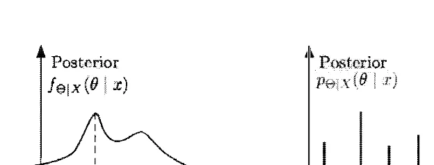
8 . 1 . A _{summary of a inference modeL The} distri but ion of the e and observation X , or

and cond i tional Pfvl F j P D F . G i ven the val ue x of the observation X , the

is usi ng The can be used to

Sec. 8. 1 Bayesian Inference and the Posterior Distribu tion 413

Summary of Bayesian Inference

•

We start with a prior distribution

pe

or

ie

for the unknown random

variable

e.

•

We have a model

PX le

or

iX le

of the observation vector X .

•

After observing the value

x

of X , we form the posterior distribution

of

e,

using the appropriate version of Bayes' rule.

Note that there are four different versions of Bayes' rulp. which we repeat

here for easy reference. They correspond to the different combinations of discrete

or continuous

e

and X . Yet. all four versions are syntactically similar: starting

from the simplest version

(

all variables are discrete

)

. we only need to replace a

PMF with a PDF and a sum with an integral when a continuous random variable

is involved. Furthermore, when

e

is multidimensional. the corresponding sums

or integrals are to be understood as multidimensional.

The Four Versions of Bayes' Rule

•

e

discrete, X discrete:

•

e

discrete, X continuous:

(0

_I

) - pe (O)ixle (x

I 0)

Pe lx x

-L

pe (

0'

) i x Ie (x

I 0')

(Jf •

8

continuous, X discrete:

414 Bayesian Statistical Inference Chap. 8

Let us illustrate the calculation of the posterior with some examples.

Example 8.2. Romeo and Juliet start dating, but Juliet will be late on any date by a random amount X, uniformly distributed over the interval [0,

OJ.

The parameter 0 is unknown and is modeled as the value of a random variable e, uniformly distributed between zero and one hour. Assuming that Juliet was late by an amount

x

on their first date, how should Romeo use this information to update the distribution of 8?

Here the prior PDF is

!e (O)

=

{

1 ,

0, if otherwise, ° � 0 � 1 , and the conditional PDF of the observation is

Sec. 8. 1 Bayesian Inference and the Posterior Distribution 415

Example

8.3.

Inference of a Common Mean of Normal Random

Vari­

ables.

We observe a collection X =

(

Xl , . . . , X

n)

of random variables, with an unknown common mean whose value we wish to infer. We assume that given the value of the common mean, the Xi are normal and independent, with known vari­ ances

(7?, . . . , (7�.

In a Bayesian approach to this problem, we model the common mean as a random variable

8,

with a given prior. For concreteness, we assume a normal prior, with known mean

Xo

and known variance

(75.

Let us note, for future reference, that our model is equivalent to one of the form

i

=

1,

. . . , n,

where the random variables

8, WI , . . . , W

n

are independent and normal, with known means and variances. In particular, for any value

8,

E[Wd

=

E[Wi 1 8

=

8]

= 0,

A model of this type is common in many engineering applications involving several independent measurements of an unknown quantity.

and

According to our assumptions, we have

{

(8

-

XO)2

}

!e (8)

=

CI .

_exp

-

2(75 '

!XIS(X

1 9)

= c, . exp

{

-

.

. .

exp

{

-

,

where

Cl

and

C2

are normalizing constants that do not depend on

8.

We invoke Bayes' rule,

(8

I

x

)

_

_-

!e (8)!xle(x I 8)

J

!e(8')!xle(x I 8') d8'

'

and note that the numerator term,

_{!e (8)!xle(x}

I 8), is of the form

{

n

_(Xi

_-

₈₎

₂

}

CIC2

.

exp

-

L

2(72 .

i=O

t

After some algebra, which involves completing the square inside the exponent, we find that the numerator is of the form

where

m = n

d

.

exp

{

_

(8

2

} ,

L

Xi/(7;

i=O

_n

v =

n

1

L

1/(7;

L

1/(7;

416 Bayesian Statistical Inference Chap. 8

and

d

is a constant, which depends on the Xi but does not depend on O. Since the

denominator term in Bayes' rule does not depend on

0

either, we conclude that the posterior PDF has the form

{ (0

-

m)2

}

f

e I x

(0 I

x)

=

a . exp

-

_2v

'

for some normalizing constant a , which depends on the Xi , but not on O. We

recognize this as a normal PDF, and we conclude that the posterior PDF is normal with mean

m

and variance

v.

As a special case suppose that 0'

5

, O'

i

, . . . , O'

�

have a common value

0'2.

Then,

the posterior PDF of 8 is normal with mean and variance

Xo

+ . . . +

Xn

n + l

v =

--

n + l

0'2

,

respectively. In this case, the prior mean Xo acts just as another observation, and

contributes equally to determine the posterior mean

m

of 8. Notice also that the standard deviation of the posterior PDF of 8 tends to zero, at the rough rate of

1/ JTi" as the number of observations increases.

If the variances 0'

7

are different, the formula for the posterior mean

m

is still

a weighted average of the X i , but with a larger weight on the observations with

smaller variance.

The preceding example has the remarkable property that the posterior

distribution of

e

is in the same family as the prior distribution, namely, the

family of normal distributions. This is appealing for two reasons:

(

a

)

The posterior can be characterized in terms of only two numbers, the mean

and the variance.

(

b

)

The form of the solution opens up the possibility of efficient

recursive

inference.

Suppose that after

Xl , . . . , X n

are observed, an additional

observation

Xn+1

i

s

obtained. Instead of solving the inference problem from

scratch, we can view

_{fSlxl , ... ,Xn}

as our prior, and use the new observation

to obtain the new posterior

_{fSlxl, ... ,Xn,Xn+l '}

We may then apply the

solution of Example

8.3

to this new problem. It is then plausible

(

and can

be formally established

)

that the new posterior of

e

will have mean

Sec. 8. 1 Bayesian Inference and the Posterior Distribution 417

Example

8.4.

Beta

Priors on

the

Bias of

a

Coin. We wish to estimate the probability of heads, denoted by

0,

of a biased coin. We model

0

as the value of a random variable 8 with known prior PDF

_fe.

We consider n independent tosses and let X be the number of heads observed. From Bayes' rule, the posterior PDF of

e

has the form, for

0

E

[0, 1],

felx (0

I

k)

=

cfe(O)Pxle(k

I

0)

=

d fe(O)Ok(1

_

O)n-k,

where c is a normalizing constant

(

independent of

0),

and

d

= c

G)

.

Suppose now that the prior is a beta density with integer parameters

a

>

0

and

(3

>

0,

of the form

{

B

(

1

(3)

0

0-

1

(

1

_

O)f3-1 ,

if

0

<

0

<

1,

fe(O)

=

a,

0,

otherwise,

where

B(a, (3)

is a normalizing constant, known as the Beta function, given by

B

(

a,

(3)

=

11

00- 1 (1

_

O)f3-1 dO

=

(a - I)! ((3 - I)! .

0

(a + (3 - 1)! '

the last equality can be obtained from integration by parts, or through a proba­ bilistic argument

(

see Problem 30 in Chapter 3). Then, the posterior PDF of

e

is of the form

f (0

elx

I

k)

=

d Ok+O-l(1

_

O)n-k+f3-1

B(a, (3)

,

and hence is a beta density with parameters

a'

=

k + a,

(3'

=

n

- k + (3.

o

:::; 0 :::; 1,

I n the special case where

a

=

(3

=

1,

the prior

fe

is the uniform density over

[0, 1].

In this case. the posterior density is beta with parameters

_{k + 1}

and n

- k + 1.

The beta density arises often i n inference applications and has interesting properties. In particular, if

e

has a beta density with integer parameters

a

>

0

and

(3

>

0,

its mth moment is given by

E

[

e

m

]

=

_{B(a. 8)}

1

11

om+o-l (1

_

O)f3-1 dO

0

B(a +

m, (3

)

B(a, (3)

a(a + 1) . . . (a +

m -

1)

- (a + (3)(a + (3 + 1) . . . (a + (3 +

m

- 1) '

418 Bayesian Statistical Inference Chap. 8

Example 8.5. Spam Filtering. An email message may be "spam" or "legit­ imate." We introduce a parameter

8,

taking values

1

and

2,

corresponding to spam and legitimate, respectively, with given probabilities

_pe(l)

and

_pe(2).

Let

{WI ,

.

_.

.

, wn}

be a collection of special words (or combinations of words) whose appearance suggests a spam message. For each i, let

_Xi

be the Bernoulli random variable that models the appearance of

Wi

in the message

_{(Xi =}

1 if

W1

appears and

Xi =

0 if it does not). We assume that the conditional probabilities

_{pX1le(Xi 1 1)}

and

PXile(Xi 12), Xi =

0, 1 , are known. For simplicity we also assume that conditioned on

8,

the random variables

X I, .. . ,Xn

are independent.

We calculate the posterior probabilities of spam and legitimate messages using Bayes' rule. We have

n

pe(m) IIpxi,e(xi 1m)

P(8

_{= m}

I

XI = XI, . . . , Xn = Xn) =

m = 1, 2.

�pe(j) IIpxile(xi

I

_j)

These posterior probabilities may be used to classify the message as spam or legit­ imate, by using methods to be discussed later.

Multiparameter Problems

Our discussion has so far focused on the case of a single unknown parameter.

The case of multiple unknown parameters is entirely similar. Our next example

involves a two-dimensional parameter.

Example 8.6. Localization Using a Sensor Network. There are n acous­

tic sensors, spread out over a geographic region of interest. The coordinates of the ith sensor are

_(ai,

bd .

A vehicle with known acoustic signature is located in

this region, at unknown Cartesian coordinates

8

_{= (}

8

1,

8

2)

.

Every sensor has a

distance-dependent probability of detecting the vehicle (i.e., "picking up" the vehi­ cle's signature). Based on which sensors detected the vehicle, and which ones did not, we would like to infer as much as possible about its location.

The prior PDF

_fe

is meant to capture our beliefs on the location of the vehicle, possibly based on previous observations. Let us assume, for simplicity, that

81

_{and 82 are independent normal random variables with zero mean and unit}

variance, so that

f

_{e I , 2 - 27r}

(0 0 )

- �

e

-(Oi

+

O�)/2

.

8. 1 4 19

8.2. a. sensor network.

we assume

= 1 . is

+

iE S i f/. S

Xl =

1 i

E

the numerator over

I X

... J

, . . . ,

420

POINT

HYPOTHESIS TESTING, AND THE

discuss

it

s

X

of

we

a

posterior distribution

_PSIX

(0 I x) [or

_fSlx

(0

I

the

Fig. 8.3).

a

x (O l x),

(0 I

(

8 d

i

sc

re

t

e

_),

(8

8 . 3 . Illustrat ion of the IvIAP rule for inference of a conti nuous parameter and a

8

Equivalently, the

probability an

incorrect decision [for each observation value x, as well as

overall probability

of error

over x)] .t

t To state this more precisely, let u s consider a genera] decision rule, which upon

value x, of () g(x) . Denote by (-)

I

are to 1

the decision rule the MAP rule) a correct decision ; thus, the event { I =

I}

is the same as the event

{g(X)

= ! and similarly for

gMAP.

By the definition of the rule,

E[I I

=

any possible

Sec. 8.2 _{Point Estimation, Hypothesis Testing, and the MAP Rule 421}

The form of the posterior distribution,

as

given by Bayes' rule, allows

an important computational shortcut: the denominator is the same for all

0

and depends only on the value

x

of the observation. Thus, to maximize the

posterior, we only need to choose a value of

0

that maximizes the numerator

pe (O)pxle(x

I 0)

if

e

and

X

are discrete, or similar expressions if

e

and/or X

are continuous. Calculation of the denominator is unnecessary.

The Maximum a Posteriori Probability (MAP) Rule

•

Given the observation value

x,

the MAP rule selects a value

B

that

maximizes over

0

the posterior distribution

_Pelx

(0

I

x)

(if

e

is discrete)

or

_{felx (O}

I

x)

(if

e

is continuous) .

•

Equivalently, i t selects

0

that maximizes over

0:

pe(O)Pxle (x

I

0)

pe (O)fxle (x

I

0)

fe (O)pxle (x

I

0)

fe (O)fxle (x

I

0)

(if

e

and X are discrete) ,

(if

8

is discrete and X is continuous),

(if

e

is continuous and X is discrete) ,

(if

e

and X are continuous) .

•

I f

e

takes only a finite number of val ues, the MAP rule minimizes (over

all decision rules) the probability of selecting an incorrect hypothesis.

This is true for both the unconditional probability of error and the

conditional one, given any observation value

x.

Let us illustrate the MAP rule by revisiting some of the examples in the

preceding section.

Example 8.3 (continued). Here,

8

is a normal random variable, with mean Xo

and variance

0-6.

We observe a collection X = (Xl , . . . , Xn) of random variables which conditioned on the value () of

8,

are independent normal random variables with mean () and variances

o,f

. .

. .

.

O'� .

We found that the posterior PDF is normal

E[I] � _E[IMAP], or

p (g(X)

=

8)

� P (gMAP (X) =

8) .

Thus, the MAP rule maximizes the overall probability of a correct decision over all decision rules g. Note that this argument is mostly relevant when

8

is discrete. If

422

Bayesian Statistical Inference Chap. 8

1 sponding to spam and legitimate messages, respectively, with given probabilities pe{ l ) and pe(2), and

Xi

is the Bernoulli random variable that models the appear­ ance of

_Wi

in the message

(Xi

= 1 if

_Wi

appears and

Xi

= 0 if it does not). We

have calculated the posterior probabilities of spam and legitimate messages as

n

hand, we may be interested in certain quantities that summarize properties of

the posterior. For example, we may select a point estimate,

which is a single

numerical value that represents our best guess of the value of

e.

Let us introduce some concepts and terminology relating to estimation. For

simplicity, we assume that

e

is one-dimensional, but the methodology extends

to other cases. We use the term

estimate

to refer to the numerical value

8

that

we choose to report on the basis of the actual observation

x.

The value of

8

is

Sec. 8.2 _{Point Estimation, Hypothesis Testing, and the MAP Rule 423}

The reason that

e

is a random variable is that the outcome of the estimation

procedure depends on the random value of the observation.

We can use different functions

9

to form different estimators; some will be

better than others. For an extreme example, consider the function that satisfies

g

(

x

)

=

0 for all

x.

The resulting estimator,

e

=

0, makes no use of the data, and

is therefore not a good choice. We have already seen two of the most popular

estimators:

(a) The

Maximum a Posteriori Probability (MAP)

estimator. Here,

having observed

x,

we choose an estimate () that maximizes the posterior

distribution over all (), breaking ties arbitrarily.

(b) The Conditional Expectation

estimator, introduced in Section

4.3.

Here,

we choose the estimate

{}

=

E[8 1

X

= x

l

.

The conditional expectation estimator will be discussed in detail in the

next section. It will be called there the least mean squares (LMS) estimator

because it has an important property: it minimizes the mean squared error over

all estimators, as we show later. Regarding the MAP estimator, we have a few

remarks.

(a) If the posterior distribution of

8 is symmetric around its (conditional) mean

and unimodal (i.e. , has a single maximum) , the maximum occurs at the

mean. Then, the MAP estimator coincides with the conditional expectation

estimator. This is the case, for example, if the posterior distribution is

guaranteed to be normal, as in Example

8.3.

(b) If 8 is continuous, the actual evaluation of the MAP estimate

{}

can some­

times be carried out analytically; for example, if there are no constraints on

(), by setting to zero the derivative of !elx (() I

x

)

,

_{or of log !elx (() I}

x

)

,

and

solving for (). In other cases, however, a numerical search may be required.

Point Estimates

•

An

estimator

is a random variable of the form

e

=

g(X ) , for some

function g. Different choices of

9

correspond to different estimators.

•

An

estimate

is the value

{}

of an estimator, as determined by the

realized value

x

of the observation X .

•

Once the value

x

o f X is observed, the

Maximum a Posteriori

Probability (MAP)

estimator, sets the estimate

{}

to a value that

maximizes the posterior distribution over all possible values of ().

•

Once the value

x

of X is observed, the

Conditional Expectation

424 Bayesian Statistical Inference Chap. 8

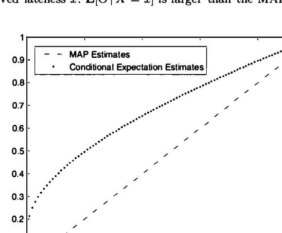
The conditional expectation estimate turns out to be less "optimistic." In particular, we have

Figure 8.4. MAP and conditional expectation estimates as functions of the observation x in Example 8.7.

Sec. 8.2 _{Point Estimation, Hypothesis Testing, and the MAP Rule 425}

In the absence of additional assumptions, a point estimate carries no guar­

antees on its accuracy. For example, the MAP estimate may lie quite far from

the bulk of the posterior distribution. Thus. it is usually desirable to also re­

port some additional information, such as the conditional mean squared error

E

[(

e

-

e)2 I X

= x

]

.

In the next section, we will discuss this issue further.

In particular, we will revisit the two preceding examples and we will calculate

the conditional mean squared error for the MAP and conditional expectation

estimates.

Hypothesis Testing

In a hypothesis testing problem,

e

takes one of

m

values,

(h , . ..

, ()m,

where

m

is usually a small integer; often

m = 2,

in which case we are dealing with a

binary hypothesis testing problem. We refer to the event

{e

=

()d

as the ith

hypothesis, and denote it by

Hi.

Once the value

x

of

X

is observed, we may use Bayes' rule to calculate

the posterior probabilities

P(8

=

()i I X

= x) =

Pelx (()i I

x

)

,

for each i. We may

426 Bayesian Statistical Inference Chap. 8

The MAP Rule for Hypothesis Testing

•

Given the observation value

x,

the

MAP

rule selects a hypothesis

Hi

for which the value of the posterior probability

P( e

= (h

I X

=

x)

is

largest.

•

Equivalently, it selects a hypothesis

Hi

for which

pe((h)Pxle(x

I

(h)

(

if

X

is discrete

)

or

pe(Oi)!xle(x

I

(h

) (

if

X

is continuous

)

is largest.

•

The

MAP

rule minimizes the probability of selecting an incorrect hy­

pothesis for any observation value

x,

as

well

as

the probability of error

over all decision rules.

Once we have derived the

MAP

rule, we may also compute the correspond­

ing probability of a correct decision

(

or error

)

,

as

a function of the observation

value

x.

In particular, if

_9MAP(X)

is the hypothesis selected by the

MAP

rule

when

X

=

x,

the probability of correct decision is

P(8

=

9MAP(X)

I X

=

x) .

Furthermore, if Si is the set of all

x

such that the

MAP

rule selects hypothesis

Hi ,

the overall probability of correct decision is

p (e

=

9MAP(X))

=

L P(e

=

Oi , X

E

Sd,

and the corresponding probability of error is

The following is a typical example of

MAP

rule calculations for the case of

two hypotheses.

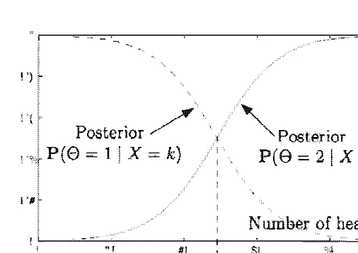
Example 8.9. We have two biased coins, referred to a..<; coins 1 and 2, with prob­

abilities of heads equal to PI and P2 , respectively. We choose a coin at random (either coin is equally likely to be chosen) and we want to infer its identity, based on the outcome of a single toss. Let

e =

1 and 8 = 2 be the hypotheses that coin 1 or 2, respectively, was chosen. Let X be equal to 1 or 0, depending on whether the outcome of the toss was a head or a tail, respectively.

Using the MAP rule, we compare pe ( 1 )Px l e (x 1 1 ) and pe (2)px le(x 1 2) , and decide in favor of the coin for which the corresponding expression is largest. Since pe (l)

=

pe (2) = 1/2, we only need to compare PX l e (x 1 1) and PX le(x 1 2), and

select the hypothesis under which the observed toss outcome is most likely. Thus, for example, if PI = 0.46, P2 = 0.52. and the outcome was a tail we notice that

and decide in favor of coin 1 .

ing to we should select which out­

come is most l ikely [this critically depends on the assumption

pe(l)

=

pe(2)

=

1/2].

Thus, if X

=

k, we should decide that ₌ 1 if

= 2

k (

)n-k k (

)n-k

PI I

-

PI > P2 1 - P2 ,

Figure 8 . 5 . The MAP rule for Example 8 .9, i n the case w here n 50,

Pi _{= 0.46, and P2 =} 0.52. It the posterior probabilities

= i l X = =

c(k) pe(i)

=

pe

(_i)

=

k

I e = i)

( 1 - i = 1 , 2,

w here c( k)

is

a. chooses the

e = i that has the largest posterior probabili ty. B ecause =

Pe (2)

= 1/2 in this example, the MAP rule chooses the hypothesis e = i for which

p�(1 _pdn-k

is The rule is to e = 1 if

k :5 k"' ,

where

k'*

= and to e = ₂ otherwise.

is

it is by a

observation space into the two disjoint sets in which each of the two hypotheses is

error is obtained by using the total probability

(8 = 1 , >

)

+ P(8 = X ::;

)

=

pe( l)

8

is a constant. of

error for a threshold- type of decision rule, as a function of the threshold k- . The

MAP rule, which in current example

, and

Threshold

8.6. A of the of error for a of decision

rule t hat e = 1 if Ie � k" and as a

of the threshold k'll' (cf. Example 8.9) . The problem data here are n = 50 ,

P i = and _P2 = 0.52. t he same as in 8 . 5. The threshold of the rule is k- = and minimizes probability of error .

The following is a classical example from com munication

[

respectively,

(b1 ,

• . • I

bn)].

We assume t hat t he two candidate signals

In is a

"energy,!l ,

ai

+ . . . + + . . . + b� . The receiver observes transmitted

, but by More it obtains the

i ₌ 1 , . . . , n,

where we assume that the Wi are standard normal random variables! independent

Sec. 8.2 _{Point Estimation, Hypothesis Testing, and the MAP Rule 429}

Under the hypothesis

e

=

1 ,

the

Xi

are independent normal random vari­

ables, with mean

ai

and unit variance. Thus,

Similarly,

From Bayes' rule, the probability that the first message was transmitted is

After expanding the squared terms and using the assumption a

i

+ . . . + a

�

bi

+ . . . +

b� ,

this expression simplifies to

The formula for

p(e

= 2 1

X

=

x

)

is similar, with the

ai

in the numerator replaced

by

b

• .

According to the MAP rule, we should choose the hypothesis with maximum posterior probability, which yields:

select

e

=

1

if

select

e

= 2 if

n n

L

aiXi

>

L

biXi,

i=l

i=l

n n

L

aiXi

<

L

b.Xi.

i=l

i=l

(If the inner products above are equal, either hypothesis may be selected.) This particular structure for deciding which signal was transmitted is called a matched filter: we "match" the received signal

(Xl ,

. .

.

,

x

n) with each of the two candidate signals by forming the inner products

_{L�=l aiXi}

and

_{L�=l biXi;}

we then select the hypothesis that yields the higher value (the "best match" ).

430

LEAST MEAN

ESTIMATION

we in more detail the conditional

8

we show that it results in the least possible mean squared error

(hence mean some of

its other properties.

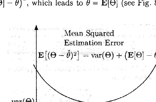
We by

mean

of e with a

con-estimation efror is random errOf

[(9

-

8)2]

is a

on and can minimized over (). this criterion, it turns out that the best possible esti mate is to set

{}

equal to

E[e] ,

as we proceed to

[(9

-we

+

uses = var(

Z)

+

(E[ Z])

_{2 1}

holds because when the constant

iJ

is subtracted froln the random variable

9,

the

by

to

{} = E[8]

Fig. 8 . 7) .

8.7: The mean squared error E

[(9

- 1 as a function of the estimate

8, is a in 8, and is m i n i mized when 8 = . The minimum value of

the mean error is var(e) .

now that we use an observation we know the

Sec. 8.3 _{Bayesian Least Mean Squares Estimation 431}

Generally, the (unconditional) mean squared estimation error associated

with an estimator

g(X)

is defined as

If we view

E[8 1 X]

as an estimator/function of

X,

the preceding analysis shows

that out of all possible estimators, the mean squared estimation error is mini­

mized when

g(X) = E[8 1 X] .t

Key Facts About Least Mean Squares Estimation

Thus,

•

In the absence of any observations,

E [(8 - 0)2]

is minimized when

0 = E[8]:

�

for all ().

•

For any given value

x

of

X, E [(8 - 0)2 1 X = x]

is minimized when

0 = E[8 I X = x] :

E

[

(8 - E[8 I X = xj) 2 1 X = x

]

< E [(8 - 0)2 I X = x] ,

for all O.

•

Out of all estimators g(X) of 8

based on

X, the mean squared esti­

mation error

E

[

(8 - g

(

X)) 2

]

is minimized when

g(X) = E[e I X] :

for all estimators g(X).

t For any given value

x

of

X, g(x)

is a number, and therefore,

which is now an inequality between random variables (functions of

X).

We take ex­ pectations of both sides, and use the law of iterated expectations, to conclude that

8

be uniformly distributed over the interval [4, 10] and suppose

we assume independent of

e.

some error W . we

x = +

W is u niformly over 1 . 1 ) and

E[e I

, we note if

4

::; e ::; 10,

(8) = Conditioned on to some 8, is same as

8 + W , and is u n iformly distributed over the interval [8 - 1 : 8 + 11 . Thus, the joint

PDF is by

(O, X) = !e (8)/xI9

=

_{6 2}

1 1

=

1

if

4

::; () ::; 1 0 and () - 1 ::; x ::; e + I , and is zero for an other values of

(

(), x). The

parallelogram in the right-h and side of is the set of which

fa,x (0, is nonzero.

8.8: The PDFs in PDF of e and X is

uniform over the shown on the

the val ue x of the random variable X = e + W, depends on x and is

represented by the l i near function shown on the right .

G iven that X = x , the posterior PDF _felx

to a

val ue x of

X

1 the mean

function of error, defined as

=

x

]

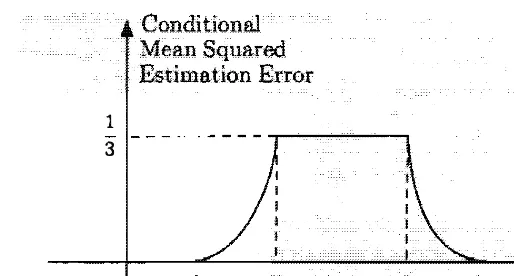
. is the It is a of x ,

i n which Juliet i s late o n the first date by

a random amount X that is uniformly distributed over the interval [0, 8j . Here,

is an unknown a over

Sec. Least Mean Squares Estinlation

1 3

8.9: The conditional mean error in 8. 1 1 , as _{a function}

of the observed va.lue _x of X . Note that certain values of the observation are more if X _{= 3, we are certain that 9} = _{4 ,}

and the conditional mean

IS

E[9 j X = I - x

x l dO = I x l '

Let us calculate the cond itional mean error for MAP

LMS estimates. Given X

=

x, for any

iJ,

we have

'" 2 '" 2 I

11

[(8

-

8) I X =

x]

= x

(8 - 8)

.

fJ l log x l d8

=

[({P-

+

8 )

2 1 ,

8

1 log x l dO

=

- iJ

+

the MAP estimate, () = X , the conditional mean error is

= +

mean

1

-2 1 log x l

( )2

I - x

log x

conditional mean errors of two are

error is

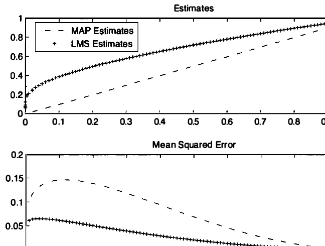
Fig. 8. 10, as functions of x . and it can be seen that the LMS estimator

uni-smaller mean squared error. This is a manifestation of t he general optimality

434

o -o 0.1

Bayesian Statistical Inference

Estimates

0.2 0.3 0.4 0.5 0.6 0.7 0.8 0.9

Mean Squared Error

0.2 0.15

f

0.1

0.1 0.2 0.3 0.4 0.5 0.6 0.7 0.8 0.9

x

Chap. 8

Figure 8. 10. MAP and LMS estimates, and their conditional mean squared errors as functions of the observation x in Example 8. 12.

Example

8. 13. We consider the model in Example 8.8, where we observe the number

X

of heads in

n

independent tosses of a biased coin. We assume that the prior distribution of

8,

the probability of heads, is uniform over

[0, 1].

In that example, we saw that when

X = k,

the posterior density is beta with parameters

Q

= k +

1 and {3

= n - k +

1 , and that the

MAP

estimate is equal to

kin.

By using

the formula for the moments of the beta density

(d.

Example 8.4) , we have

E[8Tfl I X = k] = (k + l)(k +

_{(n + 2)(n + 3) · · · (n + m +}

2) · · · (k + m)

₁₎

,

and in particular, the

LMS

estimate is

E[8 1 X = k] = k +

_{n + 2}

1

.

Given

X = k,

the conditional mean squared error for any estimate

{j

is

E [({j - 8)2 1 X = k] = {j2 - 2 {j E [8 1 X = k] + E [82 1 X = k]

= {j2

_

2 {j k +

1

+ (k + l)(k + 2) .

n + 2 (n + 2)(n + 3)

The conditional mean squared error of the

MAP

estimate is

E [(O - S)2 1 X = k] = E

[

(�

- S

r

I

X = k

]

_

�

2

_

2

�

.

k +

1

+ (k + l)(k + 2)

Sec. 8.3 _{Bayesian Least Mean Squares Estimation}

The conditional mean squared error of the

LMS

estimate is

E [(t� - e)2 1 X = k] = E [S2 I X = k] - (E[S I X = kJ)2

=

(k + 1)(k + 2)

_

(

k + 1

)

2

(n + 2)(n + 3)

n + 2

435

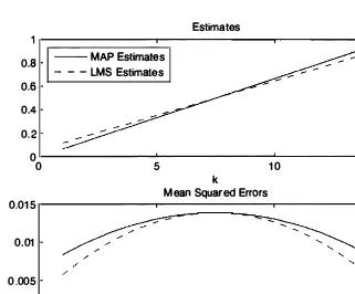
The results are plotted in Fig.

8.11

for the case of

n = 15

tosses. Note that, as in the preceding example, the

LMS

estimate has a uniformly smaller conditional mean squared error.

Estimates

0.8 MAP Estimates

- - - LMS Estimates

0.6 0.4 0.2 0

0 5 10 15

k

Mean Squared Errors

0.015

0.01

/'

"-0.005

"-0

0 5 10 1 5

k

Figure 8.11. MAP and LMS estimates, and corresponding conditional mean squared errors as functions of the observed number of heads k in n = 15 tosses

(cf. Example 8. 13).

Some Properties of the Estimation Error

Let us use the notation

e

=

E[9 I Xj,

436 Bayesian Statistical Inference Chap. 8

Properties of the Estimation Error

•

The estimation error 8 is

unbiased,

I.e., it has zero unconditional

and conditional mean:

E[e] = 0,

E[e

I X

= x] = 0,

for all

x.

•

The estimation error

e

is uncorrelated with the estimate 8:

coV(8,

e)

=

0.

•

The variance of 8 can be decomposed as

var(8)

=

var(8)

+

var(e).

Example 8. 14. Let us say that the observation X is uninformative if the mean

squared estimation error E[82]

=

var(8) is the same as var(e). the unconditional variance of e. When is this the case?

Using the formula

var(e) = var(8) + var(8),

we see that X is uninformative if and only if var

_(e)

= O. The variance of a random variable is zero if and only if that random variable is a constant, equal to its mean. We conclude that X is uninformative if and only if the estimate

_e

= E[e I X] is equal to E[e] , for every value of X.

If e and X are independent, we have E[e

_I

X

= x] = E[e] for all x, and

X

is

indeed uninformative, which is quite intuitive. The converse, however, is not true: it is possible for E[e I X

=

x] to be always equal to the constant E[e], without e and X being independent. (Can you construct an example?)

The Case of Multiple Observations and Multiple Parameters

The preceding discussion was phrased as if

X

were a single random variable.

However, the entire argument and its conclusions apply even if

X

is a vector of

random variables,

X

=

(Xl ,

. . . , Xn) . Thus, the mean squared estimation error

is minimized if we use

E[8

I Xl

. .

. . ,Xn] as our estimator, i.e.,

for all estimators

g(XI , . . .

,

X

n).

This provides a complete solution to the general problem of

LMS

estima­

Sec. 8.4 _{Bayesian Linear Least Mean Squares Estimation 437}

(a) In order to compute the conditional expectation

E[8

I Xl , " " Xn] ,

we need

a complete probabilistic model, that is, the joint PDF

fe.xl , " " Xn ,

(b) Even if this joint PDF is available,

E[8

I Xl , . . . , Xnl

can be a very

com-plicated function of

Xl , . . . , X n .

As a consequence, practitioners often resort to approximations of the conditional

expectation or focus on estimators that are not optimal but are simple and easy to

implement. The most common approach, discussed in the next section, involves

a restriction to linear estimators.

Finally, let us consider the case where we want to estimate multiple pa­

rameters

81 , . . . , 8m.

It is then natural to consider the criterion

and minimize it over all estimators

81 ,

.

. .

,

8

m

. But this is equivalent to find­

ing, for each

i,

an estimator

8i

that minimizes

E [(8i

-

8i)2] ,

so that we are

essentially dealing with

m

decoupled estimation problems, one for each unknown

parameter 8i, yielding

8i

=

E

[8

i

I Xl , . . . , Xn] ,

for all

i.

8.4 BAYESIAN LINEAR LEAST MEAN SQUARES ESTIMATION

In this section, we derive an estimator that minimizes the mean squared error

within a restricted class of estimators: those that are linear functions of the

observations. While this estimator may result in higher mean squared error, it

has a significant practical advantage: it requires simple calculations, involving

only means, variances. and covariances of the parameters and observations. It is

thus a useful alternative to the conditional expectation/LMS estimator in cases

where the latter is hard to compute.

A linear estimator of a random variable

8,

based on observations

Xl , . . . , X n .

has the form

Given a particular choice of the scalars

aI , . . . ,an ,

b,

the corresponding mean

sq uared error is

The linear LMS estimator chooses

aI , . . . , an,

b

to minimize the above expression.

We first develop the solution for the case where

n =

1 ,

and then generalize.

Linear Least Mean Squares Estimation Based on a Single Observation

We are interested in finding

a

and

b

that minimize the mean squared estimation

error

E [(8

-

aX

-

b)2]

associated with a linear estimator

aX

+

b

of

8.

Suppose

438 Bayesian Statistical Inference Chap. 8

choosing a constant

b

_{to estimate the random variable 8 - aX. By the discussion}

in the beginning of Section

8.3,

the best choice is

b =

_{E[8 - aX]}

=

E

[8

]

- a

E

_[X

]

.

With this choice of

b,

it remains to minimize, with respect to a, the expression

E

[

(8 - aX -

E

[8]

+

a

E

_[X])

2

]

.

We write this expression as

var(8 - aX)

= a

�

+

a

2a

�

+

2cov(8, -aX)

= a

�

+

a2a

�

- 2a · cov(8, X),

where

ae

and a x

are the standard deviations of 8 and X, respectively, and

cov(8, X)

=

E

[

(8 - E[8]) (X -

E

[X])

]

is the covariance of 8 and X. To minimize var(8 - aX) (a quadratic function

of a), we set its derivative to zero and solve for a. This yields

where

cov(8, X)

paeax ae

a

=

a2 _x - a2 _x = p- , ax

cov(8, X)

aeax

is the correlation coefficient. With this choice of a, the mean squared estimation

error of the resulting linear estimator

8

is given by

var(8 -

8)

= a

�

+

a

2a

�

- 2a . cov(8, X)

a2 ae

= a

�

+

p2 a

�

- 2p-paea x

ax ax

=

( 1

- p2

)

a

�

.

Linear LMS Estimation Formulas

•

The linear LMS estimator

8

of 8 based on X is

8

=

_E[8]

₊

cov(8, X) (X -

E

[X])

= E

[8]

+

P ae

(X -

E

[X])

,

var(X)

ax

where

cov(8, X)

p = _aeax

is the correlation coefficient.

Sec. 8.4 _{Bayesian Linear Least Mean Squares Estimation 439}

The formula for the linear LMS estimator only involves the means, vari­

ances, and covariance of

8

and

X.

Furthermore, it has an intuitive interpreta­

tion. Suppose, for concreteness, that the correlation coefficient

_p

is positive. The

estimator starts with the baseline estimate

E[8]

for

8,

which it then adjusts by

taking into account the value of

X - E[X] .

For example, when

X

is larger than

its mean, the positive correlation between

X

and

8

suggests that

8

is expected

to be larger than its mean. Accordingly, the resulting estimate is set to a value

larger than

E[8] .

The value of

_p

also affects the quality of the estimate. When

Ipi

is close to

1 ,

_{the two random variables are highly correlated, and knowing}

X

allows us to accurately estimate

8,

resulting in a small mean squared error.

We finally note that the properties of the estimation error presented in

Section

8.3

can be shown to hold when

8

is the linear LMS estimator; see the

end-of-chapter problems.

Example

8.15. We revisit the model in Examples 8.2, 8.7, and 8.12, in which

Juliet is always late by an amount

X

that is uniformly distributed over the interval

[0,

e],

and 8 is a random variable with

a

uniform prior

PDF Ie

(0)

over the interval

[0, 1

]

. Let us derive the linear LMS estimator of

e

based on

X.

Using the fact that

_E[X

1 8] =

e

/2 and the law of iterated expectations, the

expected value of

X

is

E[

X]

=

E [E[X

I eJ]

=

E

[�]

= =

�.

Furthermore, using the law of total variance (this is the same calculation as in Example 4.17 of Chapter 4), we have

7 v

a

r(

X)

= 144 '

We now find the covariance of

X

and 8, using the formula

and the fact

We have

cov(e,

X)

=

E[eX] - E[e] E[X],

2

( )2

1 1 1

E[e ]

= var(8) +

E[8]

=

12 +

4

=

3'

E[eX]

�

E [E[eX I ell

�

E [e E[X I ell

�

E

=

�,

where the first equality follows from the law of iterated expectations, and the second equality holds since for all

0,

440

The corresponding conditional mean squared error is calculated using the

formula derived in Example

8. 12,

and substituting the expression just derived,

{} =

(

6

/7

)

x

+

(2/7).

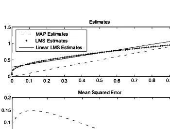
In Fig.

8. 12,

we

compare the linear

LMS

estimator with the

MAP

estimator and the

LMS

estimator

(cf. Examples

8.2, 8.7,

and

8.12).

Note that the

LMS

and linear

LMS

estimators

are nearly identical for much of the region of interest, and so are the corresponding

conditional mean squared errors. The

MAP

estimator has significantly larger mean

squared error than the other two estimators. For

x

close to

1,

the linear

LMS

Sec. 8.4 _{Bayesian Linear Least Mean Squares Estimation 441}

Example

8.16.

Linear LMS Estimation of the Bias of a Coin.

We revisit the coin tossing problem of Examples

_{8.4, 8.8,}

and 8.13, and derive the linear LMS estimator. Here, the probability of heads of the coin is modeled as a random variable

e

whose prior distribution is uniform over the interval

[0,

1] .

The coin is tossed

n

times, independently, resulting in a random number of heads, denoted by X. Thus, if

e

is equal to 0, the random variable X has a binomial distribution with parameters n and

O.

We calculate the various coefficients that appear in the formula for the linear LMS estimator. We have

E

[e

]

=

1/2,

and

E[

X

]

=

E [E[X I

en

=

E[ne]

=

%.

The variance of

e

is

1/12,

so that ue =

1/v'I2.

Also, as calculated in the previous

example,

_E[e2]

=

1/3.

If 9 takes the value 0, the (conditional) variance of X is

n

O

(

1

- 0). Using the law of total variance, we obtain

var(X) = E

[

var(X 1 9)

]

+

var

(

E[

X 1 9]

)

= E [ne(l - e)] +

var(

n

9)

n n n2

=

_{2" - "3}

+

12

n(n

+

2)

12

In order to find the covariance of X and

e,

we use the formula

n

cov(9, X) =

E

[e

X

]

-

E

[e

]

E[

X

]

=

E

[e

X

]

- 4.

Similar to Example 8. 15, we have

so that

n n n

cov(9 X)

,

= - - -

=

-3 4

12 ·

Putting everything together, we conclude that the linear LMS estimator takes the form

442 Bayesian Statistical Inference Chap. 8

The Case of Multiple Observations and Multiple Parameters

The linear LMS methodology extends to the case of multiple observations. There

is an analogous formula for the linear LMS estimator, derived in a similar man­

ner. It involves only means, variances, and covariances between various pairs of

random variables. Also, if there are multiple parameters

8i

to be estimated, we

may consider the criterion

and minimize it over all estimators

81 ,

.

.

.

, 8m

that are linear functions of the

observations. This is equivalent to finding, for each

i ,

a linear estimator

8i

that

minimizes

E [(8i - 8i)2] ,

so that we are essentially dealing with

m

decoupled

linear estimation problems, one for each unknown parameter.

In the case where there are multiple observations with a certain indepen­

dence property, the formula for the linear LMS estimator simplifies as we will

now describe. Let

8

be a random variable with mean

_J.l

and variance

a5,

and let

Xl , " " Xn

be observations of the form

where the Wi are random variables with mean

0

and variance

a;.

which rep­

resent observation errors. Under the assumption that the random variables

8,

WI , . . . , Wn

are uncorrelated, the linear LMS estimator of

8,

based on the

observations

Xl , . . . , Xn,

turns out to be

n

J.l/a6

+

LXi/a;

8

=

n

i=l

L1/a;

i=O

The derivation involves forming the function

and minimizing it by setting to zero its partial derivatives with respect to

al , . . . , an,

b.

After some calculation

(

given in the end-of-chapter problems

)

, this

results in

b =

J.l/a6

n

,

L1/a;

i=O

l/aJ

aj

=

n

j

=

1,

. .

.

, n,

L1/a;

i=O

Sec. 8.4 _{Bayesian Linear Least Mean Squares Estimation 443}

Linear Estimation and Normal Models

The linear LMS estimator is generally different from and, therefore, inferior to

the LMS estimator E[8 1

Xl , . . . , Xn].

However, if the LMS estimator happens to

be linear in the observations

Xl , . . . ,Xn,

then it is also the linear LMS estimator,

i.e.� the two estimators coincide.

An important example where this occurs is the estimation of a normal ran­

dom variable

8

on the basis of observations

_Xi

₌

8

+

Wi , where the Wi are

independent zero mean normal noise terms, independent of 8.

This is the same

model as in Example

8.3,

where we saw that the posterior distribution of 8 is

normal and that the conditional mean is a linear function of the observations.

Thus, the LMS and the linear LMS estimators coincide. Indeed, the formula for

the linear LMS estimator given in this section is consistent with the expression

for the posterior mean

{j

in Example

8.3

(

the notation

J.l

here corresponds to

Xo

in Example

8.3).

This is a manifestation of a property that can be shown to

hold more generally: if

8,

X I , . . . ,Xn

are all linear functions of a collection of

independent normal random variables, then the LMS and the linear LMS esti­

mators coincide. They also coincide with the MAP estimator, since the normal

distribution is symmetric and unimodal.

The above discussion leads to an interesting interpretation of linear LMS

estimation: the estimator is the same as the one that would have been obtained

if we were to pretend that the random variables involved were normal, with

the given means, variances, and covariances. Thus, there are two alternative

perspectives on linear LMS estimation: either as a computational shortcut

(

avoid

the evaluation of a possibly complicated formula for

E[8 1

Xj ),

or as a model

simplification

(

replace less tractable distributions by normal ones

)

.

The Choice of Variables in Linear Estimation