THE LOAD CURRENT AND VOLTAGE ESTIMATION USING INTERPOLATION METHOD IN ELECTRICAL
POWER MONITORING SYSTEM BASED ON MICROCONTROLLER ATMEGA 8535 AND PC
Marhaposan Situmorang
Abstract. The Power monitoring system has been constructed using ACS 712 as a current sensor and step down transformer as avoltage sensor which coordinated by ATMega8535 and PC. Sensors output was processed by Microcontroller into ADC value and then it was sent into PC. In PC the ADC value was estimated into load voltage and load current value using interpolation equation written in VB.6.The interpolation equation was obtained through data analysis of load voltage and load current and ADC value of current and voltage sensors which was measured manually using digital multimeter. It was observed that load voltage and current estimation using quadratic interpolation gives a higher accuracy compare with linier and third order interpolation and achieved the percentage error in the order of 1%. The result estimated power value is displayed in PC monitor in line graph and database presentation at a certain time interval.
1. INTRODUCTION
The digital KWh meter or prepayment meter hass been widely used in nearly all family housing, office and industries. The reason is caused by the cost can be saved by controlling power consumption and free from de-layed payment. Generally, in digital KWh meter, the power consumption is accumulated and cannot be displayed at a certain time interval. Former
Received 12-12-2015, Accepted 15-02-2016.
2010 Mathematics Subject Classification: 41A05, 41A10
Key words and Phrases: power monitoring, interpolation, ACS712, ATMega 8535.
researchers use ACS 712 as a current sensor and step down transformer as a voltage sensor in a digital KWh meter which is coordinated by micro-controller ATMega 8535 and sent the results into LCD [1],[2]. The sensors output voltage is converted into ADC value and then using a constant cali-bration the real load current and voltage is determined from ADC value and then current is multiplied with voltage to get the value of power. Normally, the calibration constant is achieved from sensor data sheet and was assumed to be linier.
Other researchers construct energy meter using Netduino Plus where power consumption data was stored in SD micro which can be accessed online using Website[3]. The load current and voltage is estimated using a linier calibration between sensor voltages and load current and voltage. The power consumption is accumulated at a certain time interval until the power is accessed online. By this condition, the system can be used in a power refill bussines since the power consumption can be monitored at a certain time interval. It should be note, by using a linier calibration constant to estimate load current and voltage, it would give a deviation of power value from actual value. This can be a serious problem since the consumen would pay higher than actual cost. Furthermore, it is needed that the power consumption can be monitored in real time. The real time monitoring is needed for example in power line distribution surveillance, electrical power refill service and boarding house.
On the basis of previous research, this paper discuss the monitoring system of power consumption in real time using ACS 712 as a current sensor and step down transformer as a voltage sensor coordinated by ATMega 8535 and PC. Output voltage of current and voltage sensors are converted into ADC value by ATMega 8535 and it is sent into PC using RS 232 serial standard. The VB.6 in PC estimates the load current and load voltage from ADC value using first, second and third order interpolation polynomial equation. The interpolation polynomial equation was determined through data analysis of data points which was measured manually using digital multimeter. The similar technique using calibration constant obtained from manually measrements has been applied by Kandala [5] and Adamo et al[6] in determination of moisture content percentage for peanut and soil and gives an accurate results compared with heating conventional method.
program to estimate load current and voltage. It would give the value of estimated power with such a high accuracy. Furthermore, the VB.6 program in PC can display the results in a line graph and database presentation
2. METHODOLOGY
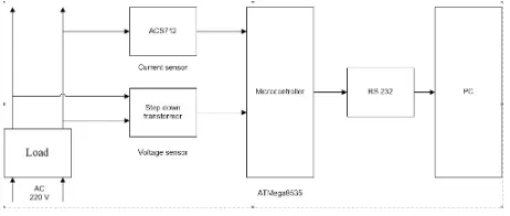
The measurement system is sketched in Fig.1. The load current and voltage is converted by sensors into voltage of 0 to 5 V and then is directed as an inputs into microcontroller. Microcontroller convert the voltage into 10 bit ADC in decimal value from 0 to 1023 and then is sent into PC using serial standard RS 232. The ADC value is then converted into load current and voltage using interpolation equation which was determined from data analysis of data points obtained from manually measurements of load current and load voltage and sensors output voltage using digital multimeter. The interpolation equation was written in VB.6 program to estimate the load current and load voltage and to calculate the power. The results was displayed in PC monitor in a line graph and database presentation using Microsoft Access.
Figure 1: Block Diagram of measurement system
2. The Polynomial Interpolation theory
Generally, data obtained from measurements are in discrete value at a certain points suh as (x0, y0),(x1, y1), . . . ,(xn−1, yn−1),(xn, yn). If we want
to find the value of y at any other value of x (other than data points) we need f(x) a polynomial of ordern passing through n+ 1 data points. The value achieved by using polynomial of order n passing through n+ 1 data points is called polynomial interpolation.
Given two data points (x0, y0) and (x1, y1), we want to construct a first
Assume the linear interpolant is given by:
f1(x) =b0+b1(x−x0) (1)
at x = x0, f1(x0) = f(x0) = b0 +b1(x0x0) = b0 so b0 = f(x0) at x =
x1, f1(x1) =f(x1) =b0+b1(x1x0) =f(x0) +b1(x1x0) givingb1= f(xx11)fx(0x0) and the linear interpolant can be expressed as
f1(x) =f(x0) + f(x1)f(x0)
Hence the quadratic interpolant can be expressed as:
f2(x) =f(x0) +
b3 =f(x3, x2, x1, x0) =
The Eqn.(2),(4) and (5) will be used to estimate load current and load voltage by applying data points of ADC value of current sensor and voltage sensor in Table 1.
3. IMPLEMENTATION
1. The measurement of load current, voltage and sensor voltage.
The load current, voltage and sensors voltages are measured using Digital Multimeter Fluke 189 after electricity 220 V AC is connected into measurement system in Fig.1. The measurements were repeated with the variation of power consumption value using 25, 40, 100 and 200 Watt light bulb and 350 Watt electric iron. Since the light bulbs and electric iron consist of pure resistance, the cos phi factor equal 1 and there is no phase difference between current and voltage. The ADC value of sensors output voltage was calculated using expression:
ADC value = Sensor output voltage
5V 2
10 (6)
All data points of load current and voltage and ADC value of sensor output voltage is shown in Table 1.
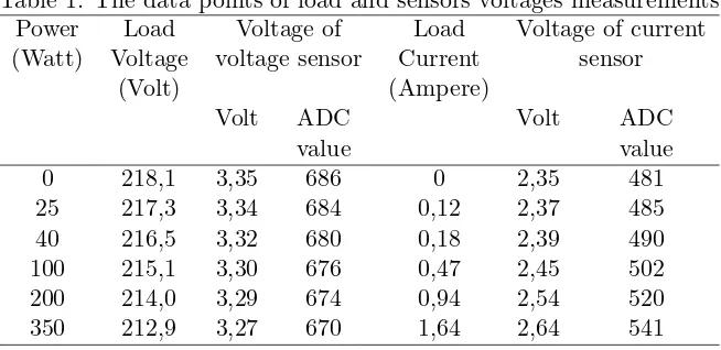
Table 1: The data points of load and sensors voltages measurements Power Load Voltage of Load Voltage of current (Watt) Voltage voltage sensor Current sensor
(Volt) (Ampere)
Volt ADC Volt ADC
value value
0 218,1 3,35 686 0 2,35 481
25 217,3 3,34 684 0,12 2,37 485
40 216,5 3,32 680 0,18 2,39 490
100 215,1 3,30 676 0,47 2,45 502
200 214,0 3,29 674 0,94 2,54 520
2. The determination of load voltage interpolation equation
The load voltage interpolation equation was determined using data points in Table 1 of ADC value of voltage sensor (x) and load voltage value (y) at a certain power value. Linear interpolation equation is determined using two data points. The first point of the ADC value of voltage of voltage sensor x0 = 686 and load voltage value y0 =f(x0) = 218,1V at zero Watt
power consumption. The second point of ADC value of voltage of voltage sensor x1 = 670 and load voltage value y1 =f(x1) = 212,9V at 350 Watt
power consumption. The calculation using Eqn. 2 gives value ofb0= 218,1
andb1 = 0,325 and the equation of linear interpolation can be expressed as:
f1(x) = 218,1 + 0,325(x686) (7)
Quadratic interpolation is determined using three data points of Table 1 at 0, 100 and 200 Watt power consumption. The three data points are
x0 = 686, y0 = f(x0) = 218,1V;x1 = 676, y1 = f(x1) = 215,1V;x2 =
674, y2 = f(x2) = 214,0V. The calculation using Eqn.4 gives value of
b0 = 218,1, b1 = 0,3 danb2 =−0,0208, and quadratic interpolation of load voltage equation can be expressed as:
f2(x) = 218,1 + 0,3(x686)0,0208(x686)(x676) (8)
Third order interpolation is determined using four data points of Table 1 at 0, 100, 200 and 350 Watt power consumption. The four data points are x0 = 686, y0 = f(x0) = 218,1V;x1 = 676, y1 = f(x1) = 215,1V;x2 =
674, y2 = f(x2) = 214,0V and x3 = 670, y3 = f(x3) = 212,9V. The
calculation using Eqn. 5 gives values of b0 = 218,1, b1 = 0,3 dan b2 = −0,0208 dan b3 = −0,000104, and third order interpolation equation of load voltage can be expressed as:
f3(x) = 218,1 + 0,3(x686)0,0208(x686)(x676)0,00104(x686)(x676)(x674)
as: f1(x) = 0.325x4.87 with residual 0,48 and quadratic equation such as
f2(x) = −0,0036x2+ 5,282x1685,6 with residual 0,43. One data point in Table 1 with ADC value 680 which is not included in interpolation will be used as data point for accuracy check. The ADC value of 680 was then substituted into both linear and quadratic curve fitting equation to get the exact value and givesy= 216,0V. On substitution the ADC value 680 into Eqn.(7) gives the estimated y value such as y= 216,15V and into Eqn.(8) gives the estimated y value such asy= 215,8V. The absolute error was ob-tained such as 216,0216,15V =−0,15V and 216,0215,8 = 0,2V and finally the percentage error is calculated such as 0,2/216×100% = 0.09%. The quadratic interpolation therefore gives a high accuracy and then Eqn,(8) is written in VB.6 to estimate load voltage.
3. The determination of load current interpolation equation
The load current interpolation equation is determined using data points of Table 1 of ADC value of voltage of current sensor (x) and load current value (y) at a certain power value. Linier interpolation equation is deter-mined using two data points. The first point of the ADC value of voltage of current sensor x0 = 481 and load current value y0 = f(x0) = 0A at
zero Watt power consumption. The second point of ADC value of voltage of current sensor x1 = 541 and load current value y1 = f(x1) = 1,64A at
350 Watt power consumption. The calculation using Eqn. 2 gives value of
b0 = 0 andb1 = 0,0273, and the equation of linear interpolation to estimate
load current can be expressed as:
f1(x) = 0 + 0,0273(x481) (10)
Quadratic interpolation is determined using three data points of Ta-ble 1 at 0, 100 and 200 Watt power consumption. The three data points are x0 = 481, y0 = f(x0) = 0A;x1 = 502, y1 = f(x1) = 0,47A;x2 =
520, y2 = f(x2) = 0,94A. The calculation using Eqn.4 gives value of
b0 = 0,0, b1 = 0,0223 dan b2 = 0,000097, and a quadratic interpolation
equation to estimate load current can be expressed as:
f2(x) = 0,0223(x481)0,000097(x481)(x502) (11)
Third order interpolation is determined using four data points of Ta-ble 1 at 0, 100, 200 and 350 Watt power consumption. The four data points are x0 = 481, y0 =f(x0) = 0A;x1 = 502, y1 =f(x1) = 0,47A;x2 =
520, y2 =f(x2) = 0,94A and x3 = 541, y3 =f(x3) = 1,64A. The
b3 = 0,0000015, and third order interpolation equation of load voltage can
be expressed as:
f3(x) = 0,0223(x481)0,000097(x481)(x502)0,0000015(x481)(x502)(x520)
(12) In order to check the validity of above equations, ADC value From Table 1 was substituted into Eqn. (10), (11) and (12) and then the results of estimation value (yinterpolation) was compared with the value ofyin Table 1 (measured manually). It was found that the estimation value using Eqn. (11) gives a value close to the measured value and using Eqn. (10) and (12) the estimation gives a great discrepancy with the measured value. Accuracy check was conducted using an exact value ofy estimated using basic fitting curve in MatLab R 2010a. The curve was plotted using data points of all ADC value of voltage of current sensor (xi) and all load current value (yi) in Table 1 and the curve was fitted to obtain linear and quadratic equation. Curve fitting gives a linear equation such as: f1(x) = 0,0268x12,949 with
residual 1,13 and quadratic equation such as f2(x) = 0,00149x20,125x+
25,856 with residual 0,03. Since the residual is smaller in quadratic equation compared with linear equation it is concluded that the exact value will be achieved using quadratic equation. One data point in Table 1 with ADC value 490 which is not included in interpolation will be used as data point for accuracy check. The ADC value of 490 was then substituted into quadratic curve fitting equation to get the exact value and gives y = 0,192A. On substitution the ADC value 490 into Eqn.(11) gives the estimated y value such asy= 0,190A. The absolute error was obtained such as 0,1920,190 = 0,002Aand finally the percentage error is calculated such as 0,002/0,192× 100% = 1,0%. The quadratic interpolation therefore gives a high accuracy and Eqn, (11) is written in VB.6 to estimate load current. The interpolation method is preferred because it just only needs a small data points compare with curve fitting using MatLab.
4. SOFTWARE DESIGN
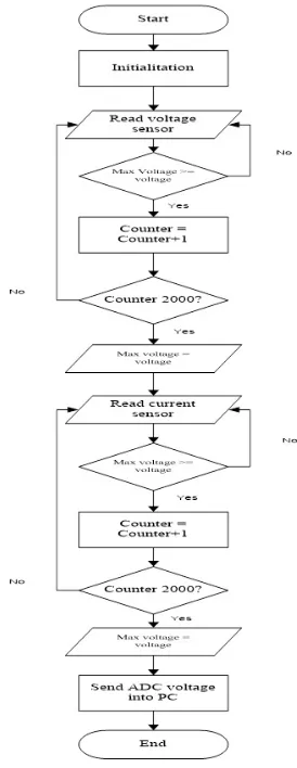
is read and after that the ADC value of voltage of current sensor is then read. Two variables that have been read finally is sent into PC. The flow chart of Codevision AVR program in microcontroller is shown in Fig. 2.
Figure 2: Flow chart program in microcontroller.
current and voltage and also to calculate power and finally to display result into line graph is written as:
j= j + 1
If (arus<= 481) Then arus = 0
Else arus = (0.0223∗ (arus 481)) + (0,000097∗(arus 481) ∗ (arus 502))
End If
arus = Round(arus, 5) ch1(j, 3) = arus
MSChart1.ChartData = ch1 MSChart1.ChartType = 3
tegangan = 218.1 + 0.325 ∗ (tegangan 686) 0,0208 ∗ (tegangan 686) ∗ (tegangan 676)
tegangan = Round(tegangan, 2) ch2(j, 3) = tegangan
MSChart2.ChartData = ch2 MSChart2.ChartType = 3
daya = arus ∗tegangan daya = Round(daya, 2) ch3(j, 3) = daya
MSChart3.ChartData = ch3 MSChart3.ChartType = 3
5. RESULTS AND DISCUSSION
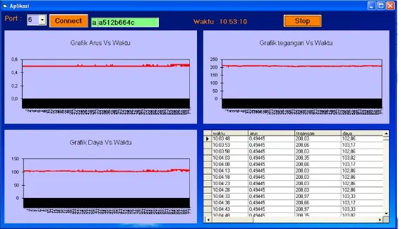
are in accordance with the power monitoring purposes so that the power value at a certain time interval can be achieved. Line graph and database of current, voltage and power presentation with the power consumption in the order of 100 Watt are shown in Fig. 4.
Figure 3: Monitoring presentation at 100 Watt power consumption
The presentation of current, voltage and power in a line graph and database as shown in Fig.4, gives a chance to monitor and control the power consumption into a minimum value so the cost can be saved. For the purpose of power line distribution surveillance, a line graph presentation is suitable since the line graph can give an exact value of time interval when the power consumption changes. Furthemore, the power value in database which is tabulated in discrete values gives a chance to modify the table record to include the price in database so the system can be used in energy refill service.
6. CONCLUSION
REFERENCES
1. Husnawati, Pasarella R., Sutarno, Rendyansyah,2013. Perancangan dan simulasi energy meter digital satu fasa menggunakan sensor arus ACS712, JNTETI,Vol.2, No. 4, November, pp 307-315.
2. Setiono A., Suharto, 2006. Prototipe applikasi KWh meter digital meng-gunakan mikrokontroler ATMega8535 untuk ruang lingkup kamar, Jurnal Ilmu Pengetahuan dan TeknologiTELAAH, Volume 26, November, pp. 32-39
3. Nirmalasari I., Putra A.E., Prastowo B.N.,2015. Purwarupa alat ukur daya listrik berbasis Netduino Plus, IJEISS, Vol.5, No.1, April, pp.21-30.
4. Chapra S.C., Canale R.P.,1996. Metode Numerik. Erlangga,Jakarta. 5. Kandala C.V.K.,2004. Moisture Determination in Single Peanut Pods by
Complex RF Impedance Measurement, IEEE Transaction on Instrumen-tation and Measurement, Vol.53, No.6, December, pp.1493-1496.
6. Adamo F.,Andria G.,Attivissimo P. and Giaquinto N.,2004. An Acoustic Method for Soil Measurements, IEEE Transaction on Instrumentation and Measurement, Vol.53, No.4, August, pp.1493-1496.
Marhaposan Situmorang: Physics Department, FMIPA University of Sumatera
Utara, Postal Code 20251, Medan, Indonesia.