Gram-Schmidt
Forward-Backward Generalized
Sidelobe Canceller
KEH-CHIARNG HUARNG
Ind ustrial Technology Re search Institute Thiwan
CHIE'" -CHUNG YEH National Taiwan University
Addressed here is the the discrete-time and the continuous-time re<un;ive least-squares (RLS) modified Gram-Schmidt orthogonallzation (MGSO) algorithms for forward-backward (FB) generali7.ed sidelohe cancelling (GSC) adaptive beamformen;. The FB-GSC requires processing each input data twice, forward and coQjugated backward, and hence its adaptation would require a rank-two update each time. This paper first derives a discrete-time rank-two-update RLS MGSO algorithm for this purpose. Then, by imposing the coQjugate symmetry constraints, the backward data processing can be removed without any loss and the complex-valued algorithm can he further transformed inlo an equivalent real-valued algorithm. Therefore, significant computation savings can he achieved. Also described here is the continuous-time RLS MGSO algorithms for the FB-GSC and Ihe coQjugate symmetric FB-GSC. Computer simulations of Ihe FB-GSC and the forward-only GSC are presented.
Manuscript received July 7, 1992; revised January 11, 1993. IEEE Log No. T-AES/30/l/13049.
Authors' addresses: K. C. Huamg, Computer and Communication Research Laboratories, Industrial 'Technology Research Institute, Hsinchu, Taiwan, KO.C.; C. C. Yeh, Department of Electrical Engineering, National Taiwan University, Thipei, Thiwan, R.O.C
0018-9251/94i$4.00 @ 1994 IEEE
I. IN TRODUCTION
Various adaptive beamformers [1) have been developed using the sample covariance matrix which is the maximum likelihood estimation (MLE) of the ensemble covariance matrix for Gaussian array inputs.
By noting the property that the covariance matrix of
the input vector of a centro-symmetric antenna array is Hermitian persymmetric, Nitzberg proposed utilizing the Hermitian per symmetric MLE of the covariance
matrix to improve the convergence rate of adaptive
beamforming [2). Furthermore, when combined with spatial smoothing, the Hermitian persymmetric MLE can decrease the number of the subarrays required for suppressing multi path interference [12, 15). T he Hermitian persymmetric MLE is formed by averaging the sample covariance matrices of the forward inputs and the conjugated backward inputs. T he forward-backward (FB) averaging, however, increases the computational load of the weight update of adaptive beamforming sincc each input vector is processed twice, forward and conjugated backward. To remedy this problem, [12] proposed two computation-saving methods, onc for the direct-form adaptive beamformer and the other for the generalized side10be canceller (GSC) [11).
As well known, the GSC is superior to the direct-form adaptive beamformer in the aspect that the GSC can easily implement multiple linear constraints and can transform the constrained minimum variance criterion into an unconstrained interference cancellation problem. 'Therefore, the
sidelohe cancelling weight vector can be updated by applying the recursive least-squares (RLS) algorithms which converge faster than the gradient-based algorithms, such as the least mean square (LMS) algorithm. The FB update of the sidelohe cancelling weight vector using the RLS algorithm has been discussed in [12]. However, it is difficult to implcment the direct update of the sidclobe cancelling weight vector in a modular structure which is desirable in adaptive signal processors.
From the viewpoint of fast convergence rate and modular implementation, the RLS modified Gram-Schmidt orthogonali7.ation (MGSO) is a
preferable approach to realize the interference
cancellation in the GSC [4-7). In the configuration of the GSC with a MGSO processor, it is the MGSO weights, instead of the GSC sidelobe cancelling weight vector, to be adapted. Both the discrete-time
and continuous-time rank-one-update RLS MGSO algorithms have been developed in [3) and [13),
respectively, which arc suitable for the forward-only
GSc. In realizing the FB adaptive beamforming,
rank-twa-update hecomes necessary due to the addition of the backward data. In this paper, we will first derive a rank-two-update RLS MGSO algorithm for the discrete-time FB-GSC. To reduce
the computational load, we will apply the conjugate symmetry constrained FB-GSC method [12] and then transform the complex-valued rank-two-update algorithm into an equivalent real-valued algorithm.
h to the continuous-time FB-GSC, we also derive a continuous-time rank-two-update RLS MGSO algorithm and then further develop a computation-saving algorithm by using the conjugate symmetry constrained FB-GSC method.
II. BASIC CONFIGURATIONS
A. Forward-Only GSC
Let us consider a K -element antenna array with the input vector
where I denotes transpose. The output of the adaptive
beamformer is formed by
yet) = wH (t)x(t) (1)
where H denotes complex conjugate transpose and wet) is a K x 1 array weight vector. According to the
linearly constrained minimum variance criterion, the optimal array weight vector at time t is determined by
(2)
subject to the constraint
CHw(t) = f (3)
where 0 < e < 1 is the forgetting factor, C is a K x M
matrix consisting of M linear constraint vectors, and f is an M x 1 vector containing the constraint values.
The linearly constrained beamforming described above can be easily implemented by the GSC. In the
GSC, the array weight vector is expressed as
wet) = Wq -8wa(t) (4)
where Wq is a K x 1 fixed quiescent beamtormer
defined as
8 is a K x N, N = K -M, signal blocking matrix of full column rank satisfying
CH8 = OMxN
and wa(t) is an N x 1 adaptive sidelobe cancelling
weight vector. In (6), the symbol 0 denotes a zero matrix (or vector) with the subscript indicating the size.
(5)
(6)
With the GSC model of (4), the beamformer output is given by
yet) = d(t) - wf/ (t)u(t) (7) where
d(t) = w
:
x(t) u(t) = 8Hx(t).(8)
(9)
In the above, d(t) is the 1 x 1 quiescent beamformer
output and u(t) is the N x 1 sidelobe canceDing signal
vector. By the minimum variance criterion (2), the sidelobe cancelling weight vector wa(t) is determined by
I
min
Ee-r
Id(r) -wf/ (t)u(r) 12.W.(I) r=O (10)
The determination of wa(t) in the GSC is an "unconstrained" least-squares optimization problem and its update can be achieved by using the RLS
algorithms.
B. Forward-Backward GSC
If the spatial distribution of the antenna elements are centro-symmetric, e.g., an equispaced line array, the phase response vector of the array elements to the far-field narrowband signal source would be in the form of conjugate symmetry for the phase reference point chosen at the array geometric center. That makes the characteristics of the impinging signals remain unchanged in the conjugated backward input vector
Xb(t) = [xK(t), ... ,x2(t),xj(t»)' (11) where * denotes complex conjugate and the subscript
b denotes "backward". Therefore, the backward data can be incorporated with x(t) to adapt the array weight vector. In the FB configuration, the array weight vector, subject to the constraint equation (3),
is determined by
It has been shown in [2 and 12] that as compared with the forward-only method, the FB method can significantly improve the performance of adaptive beamforming.
The GSC realization of the forward-backward beamformer (FB-GSC) is depicted in Fig. 1. In the figure, we have defined
db(t) = w
:
Xb(t) (13)Ub(t) = 8Hxb(t) (14)
where db(t) is the 1 x 1 backward quiescent
beamformer output and Ub(t) is the N x 1 backward
sidelobe cancelling signal vector. It is convenient to denote the FB quiescent beamformer output vector and the FB sidelobe cancelling signal matrix as
d(t) = [d(t), db (t»)' U(t) = [U(t),Ub(t)]
(15) (16)
ty(t)
Fig. 1. FB-GSC.
Fig. 2 Configuration of GSC with MGSO processor.
where d(t) is 2 x 1 and U(t) is N x 2. Then the
forward and the backward beamformer outputs can be written as a 2 x 1 vector yet), which is given by
y/(t) = d/(t) -w�/(t)U(t). (17) According to (12), the side lobe cancelling weight vector wa(t) is determined by
t
min
L:
�t-1"ll
d/(r) -w�(t)U(r)112 (18) w.(t) 1'=0where 11·11 denotes the Euclidean norm. Note that the addition of the backward data is solely for the purpose of improving the adaptation of weights. The desired beamformer output yet) is still computed from the original forward input, i.e.,
yet) = [1,O]y(t).
The adaptation of wa(t) in the FB-GSC described by (18) involves a rank-two update each time. The application of the RLS algorithm to the direct adaptation of Wa (t) for the FB-GSC has been discussed in [12]. However, the RLS MGSO would be more preferable due to its modularity. We derive a rank-twa-update RLS MGSO algorithm for the FB-GSC and utilize the conjugate symmetry criterion to develop a computation saving technique.
C. Modified Gram-Schmidt Orthogonalization
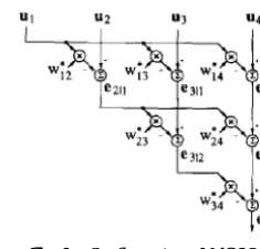
The configuration of the FB-GSC incorporating the MGSO processor is depicted in Fig. 2, which can produce the beamformer output yet) without the explicit computation of Wa(t) [3-5].
The MGSO processor has N + 1 inputs and each
input is a 2 x 1 vector, denoted Uj(t) for i = 1, ... ,N + 1. The ith MGSO input, 1 � i � N, is formed by the transpose of the ith row of the FB sidelobe cancelling signal matrix U(t), i.e.,
i =1,2, ... ,N
Fig. 3. Configuration of MGSO.
where Uj(t) and Ub,j(t) are the ith elements of u(t) and Ub(t), respectively. As to the (N + l)th MGSO input, it is the FB quiescent beamformer output vector, i.e.,
UN +1 (t) = d(t).
The detailed configuration of the MGSO processor is given by Fig. 3 with N = 3.
We now consider the "batch" MGSO processing of {ul(r)"",UN+l(r); r = 0,1, ... ,t}, from which we derive the desired RLS MGSO algorithm. In Fig. 3, the symbol ek I it 1 � i < k � N + 1, represents the residual of Uk estimated by {u I, ... , Ui} in the sense of least
squares. To be specific, ek I i represents a 2 x 1 error
vector defined as
e�1 i(r It) = u�(r) - g
�
i(t)Ui(r) (19) where Ui(r) is an i x 2 MGSO input data matrix consisting of the first i rows of U(r)Ui(r) = [Ul(r), U2(r), ... , Uj(r)]' and ItIoli(t) is the i x 1 estimation weight vector
satisfying
(20)
Note that eklo(r I t) = Uk(r) and UN(r) = U(r). From the orthogonality principle, it follows that
t
L:�t-TUi(r)ek\i(r It) = Oixl. (21)
1'=0
For the consistency of the forward and the backward notations, we denote
ek\i(r It) = [ekli(r I t),eb,k\i(r I t)]/. Comparing (19) and (20) with (18) and using UN+l(t) = d(t) and UN(t) = U(t), we find that gN +1\N(t) = wa(t) and that the FB-GSC beamformer output vector defined by (17) would be
yet) = eN+IIN(t It).
The MGSO algorithm generating ek\i(-I t) for 1 �
i < k � N + 1 is described below. From the orthogonal property of (21), one can see that {ell/-I(·I t)}!=1
forms the orthogonal basis for {UI (-)} i = I' T herefore,
(19) can be written as
i
ekli(T I t) = Uk(T)-2:Wik(t)elll-I(T It)
1=1
with the weight coefficients Wlk(t) given by
Wlk(t) = (J'lk (t)!(J'1I (t)
I
(J'lk(t) = 2:�I-Te;II_I(T I t)Uk(T) T=O
(22)
(23)
(24)
(J'1I(t) = 2:e-Tllelll_I(T I t)W (25)
T=O
which are 1 x 1 scalars. Equation (22) can be rewritten as
ekl i(T It) =
{
Uk (1') -�
wik(t)elll-I(T It)}
-wtk(t)eili_I(T It)
which is equivalent to
ekli(T It) = ekli_I(T I t) - W;k(t)eili_1(1' It). (26)
Equation (26) is applied for computing ekl i(T I t) in the MGSO as indicated by Fig. 3. Besides, instead of (24), the MGSO algorithm computes (J'jk(t) by
t
(J'ik(l) = 2:e-Te:li_I(T I t)ekli_I(T It). (27)
T=O
The equivalence of (27) to (24) can be verified by using the fact that eili-ICI t) is orthogonal to
{D1C)};:�
and hence (J'ii (t) in (25) is a special case of (J'ik (t) with k = i. In view of (27), (J'ik(t) can be termed the partial covariance betweenUjO
and Uk(-) given{UI(')};:!
while Wjk(t) is the well-known partial correlationcoefficient. T he batch MGSO algorithm requires all of the past data for computing Wik(t). In Section III, we derive an adaptive algorithm for the real-time update of the MGSO weights.
In the above descriptions, we have considered the discrete-time adaptive beamformer. A� to the continuous-time beamformer to be discussed in Section Y, all of the above equations still are applicable except that the summations should be replaced by integrations.
III. DISCRETE-TIME RANK-lWO-UPDATE RLS MGSO ALGORITHM
T he discrete-time rank-one-update RLS MGSO algorithm has been developed in [3], which is only suitable for the forward-only GSc. Following the configurations in the preceding section, we derive
in this section a rank-two-update algorithm for the FB-GSC.
Assume that at the previous instant time t -1, we have obtained the weights Wik(t -1) based on the data
Di(T), l' = O,l, ... ,t -1. Then, at the present time t, the
a priori errors ek I i (t I t -1) can be formed by applying the weights Wik(t -1) to the present inputs Ui(t). That is,
ekli(t It-I) = ekl i-let It-I) -Wikel -l)ejli_l(t It -1)
(28)
for k = i + 1,oo.,N + 1 and i = 1, ... ,N. In the
following, we derive an algorithm based on the a priori
errors to achieve the time update of weights from
Wik(t -1) to Wik(t) and obtain the a posteriori errors
ekli(t I t). Especially, eN+IIN(t I t) is the desired output. For the convenience of derivation, we first define
I
Ri(t) = 2: e-TUj(T)U[i (1') (29) T=O
I
rik(t) = 2:e-TUi(T)U;;(T) (30)
T=O
t
rik(t) = 2:e-TU:(T)Uk(T) (31)
T=O
and
[
-�I;(t)]
akli(t)= 1 (32)
where R(t) is i x i, rik(t) is i xl, rjk(t) is 1 x 1, and
ak I i (t) is (i + 1) x 1. Then the solution of (20), known as the Wiener solution, can be explicitly written as
gklj(t) = Ril (t)rik (t) (33)
and the partial covariance can also be explicitly expressed by using (24) as
(J'jk(t) = rik(t) - rt:..l,i(t)Ri-_\ (t)ri_l,k(t). (34)
With (33) and (34), we have the following derivations.
A. Time Update
To derive the time updatc of Wik(t), we first show below that thc time update of its numerator (J'ik(t) (or denominator (J'jj(t) with k = i) is given by
(J'ik(t) = �(J'ik(t -1) + e:li_1 (t I t)ek I i
-I (t I t -1).
(35) From (33) and (34), it follows that [14]
(J'ik(t) = af{;_I(t)Wik(t)akli-l(t - 1) where Wik(t) is an i x i matrix defined as
[
Ri_l(t) ri_l,k(t)]
Wik(t) = H .
ri_l)t) rik(f)
(36)
(37)
The matrix given by (37) can be decomposed as
CJ!ik(t) = �CJ!ik(t -1) + Ui(/)[V�I(t),UZ(t)]. (38)
Then substituting (38) into (36) yields (35). As to the time update of Wik(t), it is given by
Wikel) = Wik(/-l) + e;li_l (t I t)eZIJt It - l)/ITii(t). (39) To prove (39), we use (28) and (35) to obtain
O'ik(t)-Wik(/-l)O'ii(t) = e;li_l(t I t)ekl;(t
It-I).
(40)
Then (39) follows from dividing cvcry term in (40) by
O';;(t). Note that O'ii(t) in (39) can be time recursively obtained by (35).
B. Conversion Between A Posteriori and A Priori Errors
Both the time update formulas (35) and (39) require the a posteriori errors ek I i (t It). In this subsection, we present a simple approach to derive the conversion between the a priori and a posteriori errors.
The convcrsion is stated as
e�li(t It) = e�li(t It -1)ai(t) (41)
where ai(t) is a 2 x 2 conversion matrix given by ai(t) = I2x2 -U;'''ct)Ri-1(L)Ui(t). (42) The symbol I denotes the identity matrix and its subscript indicates the size. Since eklo(t It) = eklo(t I
t - 1) = Uk (t), it follows that ao(t) = I2x2' In the
literature concerning the rank-onc-updatc RLS algorithms, a would be a scalar and 1 - a is usually called the likelihood varinble.
To prove the stated conversion, we define the following (i + 1) x (i + 2) matrix
[
Ri(t) ViCt)]
.pik(t) = rik(t) u�(t) H .Then, using ( 19) and (33), we can obtain
We now decompose .pik(t) as follows:
[
�Ri(t - 1)Viet)
]
.pik(t)= �rt£(t-l) u�(t)
(43)
(44)
{
[
OiX2]
H}
X I(i+2)x(i+2)
+ hX2 [Vi (t),02x2] . (45)
TABLE I
Discrete-Time Rank-1Wo-Update Rl.S MGSO Algorithm for FB-GSC.
eilo(tll) = eilo(tlt -1) = [Ui(t), Ub,,(t)]', i = 1,2, .. , N eN+llo(tlt) = eN+llo(tlt -1) = [d(l), d,(t) I'
"o(t) = 1'<2 For i = 1,2jo .N
O',,(t) = �O' .. (t I), e:li-1(tlt)<HUII -1)
For k = i-I, , .,:V + I
ekl,(tlt -I) = ekl,_Jitlt -1) -w:k(t - l)e'I,_dtlt -I)
widt) = J1),,(t -1) + e:Hltlt)e;I,ltlt - 1)1(J'i(t) End
",U) = ",_Ill) - <H(tll)e:H(lltj!(J,,(l) e:+ti,(tlt) = e:+ti,(U - I)",(t)
End
yet) = [1, 01 eN+IN(tlt)
where O"n and Wtk are 1 x 1, ekli is 2 X 1, and OJ is 2 X 2.
Then (41) and (42) follow from the substitution of (45) into (44).
c. Order Update of Conversion Matrix
Although thc a posteriori error ek I i (t It) can be obtained from (41) using the a priori error ek I j (t I
t -1) and the conversion matrix ai (t), (42) is not applicable in real time processing. The conversion matrix should be iteratively obtained by the update of
ai(t) from Oi-I(t) for i = 1,2, ... ,N. The order update of the conversion matrix is given by
(46)
which can be derived from (42) with the inverse matrix
Ri-
\t)
substituted by [3, 14][
R�l (t) O(i-l)Xl]
1 HRil(t) = I-I + _(
)aili -l(t)aili_l(t). Olx(i-l) 0 O'ii t
(47)
Equations (28), (35), (39), (41), and (46) form the rank-two-update RLS MGSO algorithm as summarized in Thble I. Like the rank-one-update RLS algorithms, the proposed algorithm is also well suited for the triangular wavefront systolic array implementation [8-10].
IV. COMPUTATION SAVING TECHNIQUES
to eliminate the backward data computations in the FB-GSC. After that, we utilize a complex-to-real transformation to further reduce the computational load of the rank-two-update RLS MGSO algorithm.
A. Conjugate Symmetry Constrained FB-GSC
In [12], the conjugate symmetry constraint method was proposed to simplify the RLS direct update of
wa(t)
of the FB-GSC. Although with the MGSOprocessor, it is
Wik(t)
to be adapted, the conjugate symmetry constraint method still is applicable.Considering a centro-symmetric antenna array, all of the array phase response vectors and the associated derivative vectors will be complex conjugate symmetric if the phase reference point is chosen at the array geometric center. Under this circumstance, the columns of C are all conjugate symmetric if the multiple linear constraints are composed of the look-direction unit-gain constraint, the look-direction derivative constraints, and/or the known-jammer null constraints. Therefore, as described in [12], we can design a signal blocking matrix
B
with columns being conjugate symmetric. Since r is usually chosen to be real-valued,Wq
given by (5) is also conjugate symmetric. That is,.IC* = C
JB' =B
Jw; =Wq
where J is a K x K matrix defined asJ =
[:
"
J
Using J, we can rewrite (11) as
Xb(t) = .lx' (t).
(48) (49) (50)
(51)
With (51) substituted into (13) and (14), it follows from (48)-(50) that
db(t) = d' (t)
Ub(t)
=u· (t).
(52) (53)
Therefore,
Ub,j(t) = u;(t)
and each MGSO input vector would be conjugate symmetric, i.e.,Ui(t)
=[Ui(t),ui(t»)',
i = 1,2, ... ,N+ 1.
(54) Since the backward MGSO inputs are the complex conjugates of the forward MGSO inputs, the computations of the backward datadb(/)
andUb(t)
given by (13) and (14) can be avoided, which amount to K (1 + N) multiplications.From the conjugate symmetric property of (54), we find that
uW)u;;(t)
must be real-valued. Therefore,R;(t), rik(t),
and'ik(t)
defined by (29)-(31) are allreal-valued, and so is the weight vector
gkli(t)
given by (33). Accordingly, it follows from (34) that lTik(t) is real-valued and so is the MGSO weight, i.e.,(55)
Furthermore, since
gkli(t)
is real andUi(T)
is conjugate symmetric, it follows from (19) thateb,kli(T It) =
eZ1i(T
I t) and hence each error vector is conjugate symmetric, i.e.,Since every backward error is the complex conjugate of the associated forward error, thc computations involving the backward errors in (28), (35), (39), and (41) can be saved.
Furthermore, with (56) and
ao(t) = 12x2,
one may see that the conversion matrix described by (46) is not only Hermitian but also persymmetric. That is, the conversion matrix can be expressed as[ai,l1 (t) a; 21 (t)]
ai(t) =
ai,21 (t) ai,l1 (t)
'
(57) whereaj,pq(t)
represents the (p,q)th element ofaj(t).
Note thatai.l1(t)
is real sinceai(t)
is Hermitian.B. Complex-to-Real Transformation
Following the above conjugate symmetry
formulations, we propose the following transformations to further simplify the computations
(58)
(59)
where the overbars represent the transformed quantities. We show below that the above transformations convert the complex-valued parameters into real values. Using (56), the transformed error given by (58) can be shown to be
where Re and 1m denote the real and the imaginary parts, respectively. Substituting (57) into (59), the transformed conversion matrix can be shown to be
_
(aj,l1 (t)
+
Re{aj,21 (t)}
ai(t)
=Im{ai,21 (t)}
aj,l1 (t)
Im{ai,21(t)} ]
-Re{ai,21 (t)}
which is also real.
By substituting (58) and (59) into Thble
I,
we can transform the complex-valued rank-twa-update algorithm into the real-valued rank-two-update(61)
TABLE Il
Ttansformed Discrete-Time Rank-'lwo-Update RLS MGSO Algorithm for Conjugate Symmetric FB-GSC (Real-Valued)
;;;Io(tlt) = ';'Io(tlt -1) = [Re{ui(t)}. Im{ui(t)} I', i = 1,2, ... ,N
;;N+110(tlt) = ;;"'+110(111 -I) = [Re{d(t)}, Im{d(t)} l'
iio(t) = I",
For i = 1, 2, ... , l\/
u;;(l) = (U,,(t -I) + ;;:h_1(tlt);;'H(tlt -1) For k � i + 1 ... N + 1
e'I,(t11 -I) = ;;'1;_1(111 - 1) -w,.(1 -1);;'I;_I(t,t -1)
10 .. (1) = w,.(/ -1) + e:I,_l(lll)ihl;(tlt -1)/u,;(I)
Eno
iii(t) = if,_l(l) -e,li-1(llt)e:H(III)/u;;(I)
;;:+11,(111) = 1':+11;(111 -1)iii(l)
End
y(l) = [1,j] ;;N+1IN(III)
where 0-11 and Wik are 1 x 1, ekl' is 2 x 1, and (}j is 2 x 2.
algorithm listed in Thble II where we have denoted
(fu(t) =
�
a';;(t). (62)Note that only the forward data is involved in Table II. T he transformed algorithm is completely identical to the original algorithm, except that all of the quantities are transformed into real values.
Detailed comparisons between the computational loads of the algorithms given in [3], Table I, and Thblc II are given below. T he complex-valued rank-one-update algorithm given in [3] which is suitable for the forward-only GSC requires 4N2 + llN real multiplications and 2N real divisions. The complex-valued rank-two-update algorithm given in Thble I which is suitable for the FB-GSC requires
8N2 + 33N real multiplications and 4N real divisions. As to the real-valued rank-twa-update algorithm
given in Table II, it is suitable for the conjugate symmetric FB-GSC and requires 2N2 + 12N real multiplications and 2N real divisions. Therefore, Table II can save significant amount of computations
and its computational load is even less than that of the rank-one-update algorithm in [3].
Concluding this section, we remark that the FB processing required by the FB-GSC can be replaced without any loss by the forward-only processing with conjugate symmetry constraints imposed on the FB-GSC. Besides, the conjugate symmetry constraint method, when applicable, can incorporate with the complex-to-real transformation to achieve significant
computation savings for the FB-GSC with a RLS MGSO processor.
v. CONTINUO US-TIME ALGORITHMS
As to the continuous-time RLS algorithms [16], there has been a rank-one-update MGSO algorithm developed in [13]. That algorithm, however, is
only suitable for the forward-only GSc. In the continuous-time FB-GSC, the array inputs must be processed continuously together with the backward array inputs. In this section, we handle this problem and derive two continuous-time RLS MGSO algorithms, one for the FB-GSC and the other for the conjugate symmetric FB-GSC.
All of the configurations in Section II are
applicable here except that the discrete-time weighted summation
L:�=o�t-r
should be replaced by the continuous-timc weighted integrationf�
drr>.(t-r), where 0 < A is the exponential forgetting factor. Inthe continuous-time domain, there is no difference between the a priori and the a posteriori errors. Thereforc, (28) should be rewritten as
ekli(t I t) = ekli-l(t I t)- wik(t)eili-l(t I t) (63)
where Wiket) is to be adapted. To derive the time update, we rccall that Wik(t) = Uik(t)/Uii(t) and then
we have
Wik(t) = {O'ik(t) - O'ii(t) Wik (t)}/O"ii (t) (64)
where the dot indicates d / d t. From (27), the continuous-time definition of O"ik(t) is given by
Similar to (21), we have the following orthogonal property
lot
e->.(t-r)Ui(r)ekli(T I t)dT = Oi><l.To derive O'ik(t), we first note from (19) that
dekl;(T It) .H
dt = -gkli(f)Ui(T)
(65)
(66)
TABLE III
Continuous-Time Rank-'l\vo-Update RLS MGSO Algorithm for FB-GSC eilo(tlt) = [u,(t), Ub •• (t) I', i = 1,2, ... , N
eN+1Io(tlt) = [d(t), dl(t)]'
For i=1,2,
.
..
,Nf.<7;;(t) = -A<7,.(t) + II e'H(tlt) 112
For k = i + 1, " . , N + I
e'I.(tlt) = ekl,_l(tlt) -w'k(t)eil.-1(tlt)
l.W,k(t) = eili-1(tlt)eZli(tlt)!<7;;(t)
End End
yet) = [1,OJ eN+1IN(tlt)
where CTii and Will: are 1 x 1 and ekli is 2 x 1.
TABLE N
Continuous-Time RLS MGSO Algorithm for Conjugate-Symmetric FB-GSC.
€'Io(tlt) = u,(t), i = 1,2, .
.
. , N€N+llo(tlt) = d(t) For i = l,2,
...
,N1.a
..
(t) = -Aa..
(t) + 1€i1,-,(tlt)I' For k = i + 1,..
. , N + 1€'Ii(tlt) = Eklo-1(tlt) - wik(t)eiH(tlt) 1.W'k(t) = Re {eili_1(tlt)ekl,(tlt)} I a .. (t) End
End
yet) = eN+w.(tlt)
where all of the quantities are 1 X 1.
and then by using (66) and (67), we have
algorithms [13, 16]. Therefore, the continuous-time RLS MGSO algorithms are much simpler than the discrete-time ones.
If the conjugate symmetry constraints are imposed on the FB-GSC, the adaptation of Wik(t) could be even simpler. Under this condition, it has been shown in
Section IV that Wik(t) is real-valued. Furthermore, we can use the conjugate symmetric property of (56) and the definition of (62) to reduce the algorithm given in Thble III into that given in Thble N where only the forward data processing is required. Note that Thble IV is a complex-valued rank-one-update algorithm. Further note that weight update in Thble IV only requires computing the real part of eiji-l(t I t)ekji(t It) while the rank-one-update algorithm in [13] used for the forward-only GSC requires computing both the real and the imaginary parts of eili_l(t I t)ekji(t It).
11 -),(1-7')
de;"
j;(T It) •( I )d - 0
e
d ekji T t T - ,
o t i < k S; m. VI. SjMULATIONS
(68) Computer simulation results are presented in this Using (68) and applying the formula
d
t
t
d¢(t T)dt
fo
¢(t,T)dT = ¢(t,t) +10
--;jf-
dTwe can evaluate the differentiation of O'ik(t) given by (65) and obtain
O',dt) = e;ji-l (t I t)ek j i-I (t It) - ,\(J'ik (t). (69)
By substituting (69) into (64), we obtain the time update
Wikel) = e:ji_l(t I t)ekji(t I t)/O'ii(t) (70)
where ekji(t I t) is given by (63) and O'ii(t) can be generated by (69). The resulting continuous-time rank-two-update RLS MGSO algorithm is summarized in Thble III. It is of interest to note that the conversion between a priori and a posteriori errors and its order update, which are essential in the discrete-time algorithms, are absent from the continuous-time
section. We assumed a five-element equispaced line array with a look-direction constraint only. The GSC we adopted possesses a uniform-weight quiescent beamformer
Wq = [1,1,1,1,1]'
and a conjugate symmetric signal blocking matrix
-j 0 0 -1.5
0 -j -1 1
B = 0 0 2 1
0 j -1 1
j a 0 -
1
.5The look-direction desired signal source was located at the far-field broadside and was a baseband signal source modulated by a complex sinusoid carrier of frequency /0. The array element spacing was equal to one-half carrier wavelength. The base band signal
]O�-�-FB�GSC
normalized time
600 S[X)
Fig. 4. Output SINR of GSC with continuous-time RLS MGSO algorithm. For (forward-unly) GSC, rank-one-update algorithm
given in [13] is employed. As to FB-GSC, conjugate symmetry
constraints are imposed and algorithm given in Thble IV is
employed. ,\ = 0.0005 fb.
source was modeled as having flat spectrum over the bandwidth extending from -10 to Ib where
Ib == fo/20. The desired signal measured at each
array element is 20 d8 over white noise. We assume that before t == 0, the GSC with MGSO was at the interfcrence-absent steady state. At time t == 0, an equal-power uncorrelated interferer having the same frequency spectrum as the desired signal appears at the angle 30° relative to array broadside. Then the RLS MGSO processor begins to adapt the weights to achieve interference cancellation.
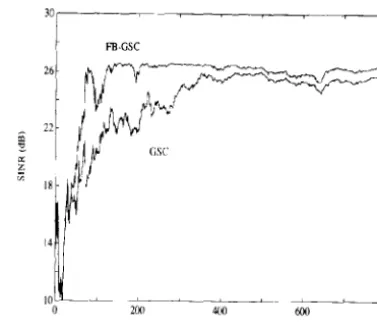
To simulate thc continuous-time RLS MGSO algorithms, we utilized thc Euler method because only the first order derivatives arc involved in the differential equations. 80th the forward-only GSC and the FB-GSC with continuous-time RLS MGSO were simulated and their output signal-to-interference-plus-noise ratios (SINR) are plotted in Fig. 4 versus the normalizcd time. A normalized time unit is equivalent to l/lb s. As to the discrete-timc RLS MGSO algorithms, we took samples of the signals used in Fig. 4. T he sampling rate Is was chosen tu be the Nyquist rate, i.e., Is == 21b. T he discretc-time forgetting factor was chosen to be � == exp( -,\/ Is), where ,\ is the continuous-time
exponential forgetting factor used in Fig. 4, to make the fading rate of past data unchanged. The output SINRs of the forward-only GSC and the FB-GSC with discrete-time RLS MGSO are plotted in Fig. 5. As shown by Fig. 4 and Fig. 5, the FB-GSC can achieve a faster convergence rate.
VII. CONCLUSIONS
We have derived the discrete-time and the continuous-time rank-twa-update RLS MGSO
lOlr ---�- -�--�-�-�--�---,
f
)4
10 o
FB·GSC
20[) 600 ROO
normalized time
Fig. 5. Output SINR of GSC with discrete-time RLS MGSO algorithm. Same scenario as Fig. 4 with Nyquist sampling rate. F or
(forward-only) GSC, rank-one-update algorithm given in [3) is (",played. As to FB-GSC with conjugate symmetry constraints,
al
g
orithm gi ven in Tabl e II is employed. � = cxp( -0.0005 /2).algorithms for the FB-GSC, which has a faster convergence ratc than the forward-only GSc. To reduce the computational load of the rank-twa-update, we eliminated the backward data processing by imposing the conjugate symmetry constraints on the FB-GSC. We further reduced the discrete-time and the continuous-time complex-valued rank-two-update RLS MGSO algorithms into a real-valued rank-twa-update algorithm and a complex-valued rank-one-update algorithm, respectively. 80th reduced algorithms for the conjugate symmetric F8-GSC require computations even less than those of the corresponding algorithms for the forward-only GSc.
REFERENCES
[1]
[2]
[3]
[4)
]5J
Compton, R. T., Jr. (1988)
Adaptive Antennas: Concepts and Performance.
Englewood Cliffs, NJ: Prentice-Hall, 1988.
Nitzberg, R. (1980)
A pplication of maximum likelihood estimation of persymmetric covariance matrices to adaptive processing.
IEEE Transactions on Aerospace Electronic Systems,
AES-16 (Jan. 1980), 124--127.
Ling, E, Manolakis, D., and Proakis, J. G. (1986) A recursive modified Gra m-Schmidt algorithm for
least-squares estimation.
IEEE Transactions on Acoustics, Speech, Signal Processing,
ASSP-34, 4 (Aug. 1986), 829--�m.
Gerlach, K. (1990)
Implementation and convergence considerations of a linearly constrained adaptive array.
IEEE Transactions on Aerospace and Electronic Systems, 26, 2 (Mar. 1990),263-272.
Gerlach, K., and Kretschmer, E E, Jr. (1990)
Convergence properties of Gram-Schmidt and SMI adaptive algorithms.
IEEE Tran,actions on Aerospace and Electronic Systems,
[6] Yuen, S. M. (1991) [12] Huarng, K. c., and Yeh, C. C. (1991)
Exact least squares adaptive beamforming using an orthogonalization network.
IEEE Transactions on Aerospace and Electronic Systems,
27, 2 (Mar. 1991), 311-330.
Adaptive beamforming with conjugate symmetric weights.
IEEE Transactions on Antennas Propagation, 39, 7 (July
1991), 926-932.
[13] Huarng, K. C., and Yeh, C. C.
[7] Yuen, S. M. (1989) Continuous-time recursive least-squares algorithms.
IEEE Transactions on Circuits and Systems, to be pUbliShed.
Algorithmic, architectural, and beam pattern issues of sidelobe cancellation.
IEEE Transactions on Aerospace and Electronic Systems,
25, 4 (July 1989), 459-471.
[14] Haykin, S. (1991)
AdJJptive Filter Theory.
[8] McWhirter, J. G., and Shepherd, T. J. (1989) Englewood Cliffs, NJ: Prentice Hall, 1991.
Systolic array processor for MVDR beamforming.
Proceedings of IEEE, 136, PI. F, 2 (Apr. 1989).
[IS] Pillai, S. U., and Kwon, B. H. (1989)
[9] Gentleman, W. M., and Kung, H. T. (1981) coherent signal identification. Forwardlbackward spatial smoothing techniques for Matrix triangularization by systolic arrays.
Proceedings of SPIE, 298 (Real-Time Signal Processing IV) (1981), 298--303.
IEEE Transactions on Acoustics, Speech, Signal Processing,
37 (Jan. 1989), 8-15.
[16] Lev-Ari, H., Kailath, T., and Cioffi, J. (1992)
[10] Ueno, M., Kawabata, K., and Morooka, T (1990) Adaptive recursive-least-squares lattice and transversal filters for continuous-time signal processing. A systolic array architecture for the Applebaum-Howells
array.
IEEE Transactions on Antennas Propagation, 38, 8 (Aug.
1990), 1310-1313.
IEEE Transactions on Circuits and Systems II: Analog and Digital Signal Processing, 39, 2 (Feb. 1992), 81-89.
[11] Griffiths, L. J., and Jim, C. W. (1982)
160
An alternative approach to linearly constrained adaptive beamforming.
IEEE Transactions on Antennas Propagation, AP-30, 1
(Jan. 1982), 27-34.
Keh-Chiarng Huarng was born in Taipei, Taiwan, Republic of China, in 1965. He received the B.S_ and Ph.D. degrecs in electrical engineering from National Thiwan University, Taiwan, in 1987 and 1992, respectively.
Currently, he is with the Computer and Communication Research Laboratories, Industrial Thchnology Research Institute, Hsinchu, Taiwan. His research interests include adaptive signal processing, magnetic recording, and
digital communications.
Chien-Chung Yeh was born in Thiwan, Republic of China, in 1954. He received the B.S. degree from National Thiwan University, Thiwan, in 1976, and the M.S. and Ph.D. degrees from the University of Pennsylvania, Philadelphia, in 1981 and 1983, respectively, all in electrical engineering.
From 1983 to 1986 he was an Assistant Professor in the Department of Electrical Engineering, State University of New York at Stony Brook, Stony Brook, NY From 1986 to 1987 he was on a leave of absence with the Department of Electrical Engineering, National Thiwan University. He became an Associate Professor at National Thiwan University in 1987, and a Professor in 1988. His current research interests include adaptive signal processing, digital signal processing and neural nctworks.
IEEE T.RANSACnONS ON AEROSPACE AND ELECTRONIC SYSTEMS VOL. 30, NO.1 JANUARY 1994