A REPLENISHMENT POLICY FOR ITEM WITH PRICE
DEPENDENT DEMAND AND DETERIORATING UNDER
MARKDOWN POLICY
Gede Agus Widyadana
Department of Industrial Engineering, Petra Christian University, Surabaya, Indonesia and PhD Student in Department of Industrial Engineering, Chung Yuan Christian University,
Chung Li 320, Taiwan
Hui Ming Wee
Department of Industrial Engineering, Chung Yuan Christian University, Chung Li 320, Taiwan
ABSTRACT
Many researches on deteriorating inventory model have been developed in recent years. This paper develops deteriorating inventory model with price-dependent demand and uses markdown policy to increase profit. Two examples are used to explain the model and some interesting results are derived. Markdown policy can increase total profit, but the best markdown time and price depend are case dependent.
Keywords: inventory, deteriorating item, markdown, price dependent demand.
1. INTRODUCTION
Some items like vegetables, milks, and fruits have deterioration characteristic. Deterioration is defined as decay, evaporation, obsolescence, loss of quality marginal value of a commodity that results in the decreasing usefulness from the original condition. The longer the items are kept in inventory, the higher the deteriorating cost. Retailer sometime uses markdown strategy to reduce their inventory and increase their profit by assuming that demand will increase with price decrease. In this study we developed a replenishment inventory model for deteriorating items and price- dependent demand. The model can be implemented for single markdown policy with different markdown time period.
Deteriorating inventory has been studied by several researches in recent decades. Goyal and Giri (2001) reviewed many literatures which studied deteriorating inventory since early 1900s. In their review, they studied some variations of deteriorating inventory with deterministic demand such as uniform demand, time-varying demand, stock-dependent demand and price-dependent demand. Kim et al (1995) presented joint price and lot size determination problems with deteriorating products using constant deterioration rate. Wee (1995) developed model for joint pricing and replenishment policy for deteriorating inventory with price elastic demand rate that decline over time. Wee (1997) studied inventory deteriorating model for price-dependent of items that have varying deterioration rate.
Modeling inventory model with markdown price and stock dependent demand is getting the attention of researchers recently. You & Shieh(2007) developed an EOQ model with stock and price sensitive demand. Their objective is to maximize profit by simultaneously determining the order quantity and selling price. They did not allow item deterioration and assumed equal period price changes.
The contribution of this paper is developing replenishment inventory deteriorating model policy when supplier used markdown policy. This paper is presented as follow. The first section presents the paper contribution and reviews the relevant literature. Section two presents calculations and details regarding the deteriorating inventory model. Two examples and experiments are presented in the third section. The fourth section offers conclusions and suggests directions for future research.
2. MODEL DEVELOPMENT Assumptions:
1. Demand increase as price is reduced. The demand has constant elasticity. The demand at time t is assumed to be
β
(
α
p
)
−ε , whereβ
andα
is positive constants.2. A single rate item with a constant rate of deterioration is considered. 3. Shortage is not allowed
4. The on hand stock deteriorates at constant rate
5. Instantaneous replenishment with continuous review order quantity 6. One time markdown price at one planning period is considered 7. Markdown price and time are known.
Notation:
It = inventory at period t T* = Optimal replenishment time
θ
= deterioration rate T P* = Optimal total profitα
= markdown rate p = Initial priceε
= increase price rate r = markdown percentageβ
= constant stock dependent parameter D = demand Q = Ordering quantity c = buying price Q* = Optimal ordering quantity RC = ordering cost T1 = Markdown offering time HC = holding costT = Replenishment time UC = cost of purchasing unit
Q
T1 T
Quantity
Time
The inventory level is illustrated in Figure 1 and it can be represented by the following
From equation (3) we know at t=T1, the quantity of inventory is equal to:
)
It can be simplified as:
)
Substitute Q from equation (6), one has:
Substitute Q from (6) and simplify the equation, one has:
The total revenue consists of the revenue before the markdown price is implemented and the revenue when the markdown is realized. The revenue equation can be obtained as:
1
Adding equation (10) and (11), and divide by the total time, the revenue rate is:
T
The total relevant cost per unit time consists of: a. Cost of placing orders =
T RC
(13)
b. Cost of purchasing units =
T cQ
Substitute Q from equation (6) to equation (14), the purchasing rate is:
))
c. Cost of carrying inventory = T
Total profit is equal to total revenue less total cost. Subtracting equation (13)-(15) to equation (12), the total profit is:
)
The objective of this case is to maximize the net profit. It is done by differentiating TP with respect to T. Differentiating TP with respect to T and substitute T1 with r*T, one has equation in
3. NUMERICAL EXAMPLE
The preceding theory can be illustrated using the numerical example. We use two examples with varying markdown time and price. The parameters are as follows:
Example 1: Suppose RC = 1000, c = 10, p = 30, HC = 0.05,
β
= 100000,θ
= 0.3,ε
= 1.8. Value of r is varying from 0.5 to 0.9 andα
is varying from 0.7 to 0.9. We solve the problem using Maple 8. The first step to solve the problem is to check the convexity and the feasibility of the solution. The second derivative is used to check this convexity. For this problem with r = 0.5 andα
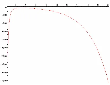
= 0.7, we check the second derivative equation in the feasible area between T=0.5 to T=20. The plot can be shown in Figure 2. Figure 2 shows that all second derivative values are negative at T, so the maximum solution is verified for this case at T=0.5 to T=20.Figure 2. Second derivative function
Table 1. Experimental result for Example 1
r = 0.5 r = 0.7 r = 0.9
α
T*Q* TP* T* Q* TP* T* Q* TP*
0.7 1.18 461.1 2886.3 1.25 433.4 2944.6 1.38 414.3 3053.3 0.8 1.29 438.5 3033.3 1.34 422.6 3047.6 1.42 412.4 3098.1 0.9 1.39 422.4 3105.3 1.42 415.5 3108.0 1.46 411.4 3122.3
Example 2: Suppose RC = 1000, c = 10, p = 30, HC = 0.05,
β
= 100000,θ
= 0.05,ε
= 1.8. In the second example, we decrease the deteriorating rate parameter (θ
) to 0.05 instead of 0.3 in Example 1. Using the same steps as Example 1, the result of this example can be seen in Table 2.Table 2. Experimental result for Example 2
r = 0.5 r = 0.7 r = 0.9
α
T*Q* TP* T* Q* TP* T* Q* TP*
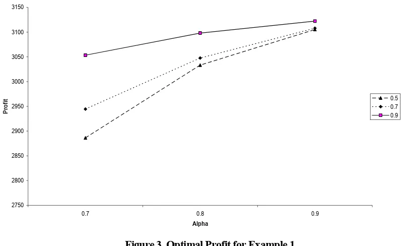
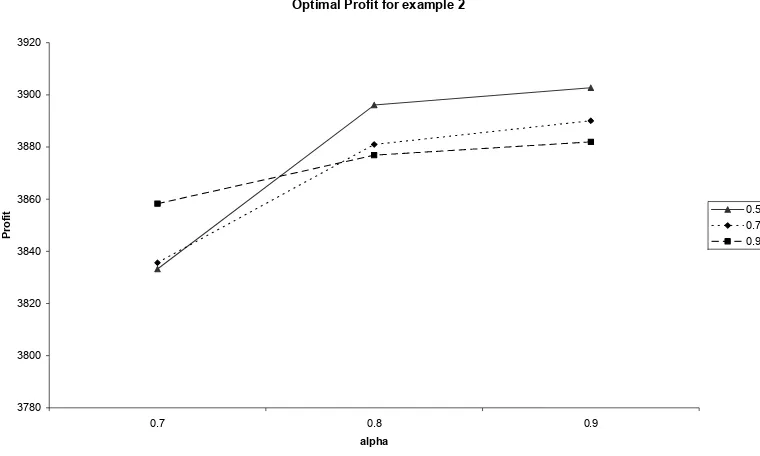
0.7 2.99 1035.0 3833.2 3.18 971.9 3835.6 3.53 930.1 3858.3 0.8 3.28 984.1 3896.1 3.42 948.1 3881.0 3.65 926.3 3876.9 0.9 3.56 948.4 3902.7 3.64 932.9 3890.1 3.75 924.2 3882.0 Table 1 and 2 show that if the value of markdown price is different at a given markdown time, the variance of the replenishment time is small but give totally different profits. The variance of total profit is bigger when markdown is applied earlier.
Optimal Profit for Example 1
2750 2800 2850 2900 2950 3000 3050 3100 3150
0.7 0.8 0.9
Alpha
Pr
o
fi
t 0.5
0.7 0.9
Optimal Profit for example 2
3780 3800 3820 3840 3860 3880 3900 3920
0.7 0.8 0.9
alpha
Pr
o
fi
t 0.5
0.7 0.9
Figure 4. Optimal Profit for Example 2
The effect of markdown price and time to optimize total profit are case dependent. In Example 1, when the price is reduced to 90% of the initial price, it dominants others markdown price at any markdown time. This condition can be seen in Figure 3. This circumstance does not happen in Example 2. We can see from Figure 4, that when markdown price strategy start at alpha equal to 0.8 and 0.9, r = 0.5 give the best profit but, when alpha equal to 0.7, then r = 0.9 give the best profit. These two examples also show when deteriorating rate is bigger, bigger markdown price and markdown time tends to derive optimal profit.
4. CONCLUSION
In this study, a deteriorating inventory model with price dependent demand under markdown policy has been developed. The optimal replenishment time and optimal ordering time were derived and two examples were shown to illustrate the model. The result demonstrates that markdown time and price give significant contribution to optimize the total profit and a policy maker must be careful to set markdown time and price because optimum policy is different for different case.
In this paper, we have not investigated the effect of another parameters of different deteriorating rate to find replenishment time and optimal profit. Different types of deteriorating function can be considered as future research. The model can also be extended to consider stochastic demand dependent rate instead of deterministic rate as in this paper.
REFERENCES
Kim. J.S. Hwang H. Shinn, 1995. An optimal credit policy to increase supplier’s profit with price-dependent functions. Production Planning and Control , 6, 45-50.
Padmanabhan G. and Vrat P. 1995. EOQ models for perishable items under stock dependent selling rate. European Journal of Operational Research, 86, 281-292.
Wee, H.M. 1995. Joint pricing and replenishment policy for deteriorating inventory with declining market. International Journal of Production Economics, 40, 163-171.
Wee, H.M. 1997. A replenishment policy for items with a price-dependent demand and varying rate of deterioration. Production Planning and Control, 8, 494-499.
You P.S. & Hsieh Y .C., 2007. An EOQ model with stock price sensitive demand. Mathematical and Computer Modelling, 45, 933-942.
You P.S. 2005. Inventory policy for products with price and time-dependent demands. Journal of the Operational Research Society 56, 870-873.
Appendix A : The derivation of equation (16)
Topt
RC
T
2c
β
(
−
p
(−ε)+
p
(−ε)e
(r Tθ)−
(
α
p
)
(−ε)e
(r Tθ)+
(
α
p
)
(−ε)e
(Tθ))
T
2θ
+
:=
c
β
(
p
(−ε)r
θ
e
(r Tθ)−
(
α
p
)
(−ε)r
θ
e
(r Tθ)+
(
α
p
)
(−ε)θ
e
(Tθ))
T
θ
hc
−
+
β(−p(−ε) + p(−ε)e(r Tθ) − (αp)(−ε)e(r Tθ) + (αp)(−ε)e(Tθ))(e(−r Tθ) − 1)
θ2
−
β (e(−r Tθ) + r Tθ − 1)p(−ε)
θ2
−
T2 hc
−
β(p(−ε)rθe(r Tθ) − (αp)(−ε)rθe(r Tθ) + (αp)(−ε)θe(Tθ))(e(−r Tθ) − 1)
θ2
−
β(−p(−ε) + p(−ε)e(r Tθ) − (αp)(−ε)e(r Tθ) + (αp)(−ε)e(Tθ))re(−r Tθ)
θ +
β(−rθe(−r Tθ) + rθ)p(−ε)
θ2
−
/T
hcβe(−Tθ)p(−ε)α(−ε)(−e(Tθ) + e(−θ(r T − 2T)) − Tθe(Tθ) + θr Te(Tθ))
T2θ2
hcβe(−Tθ)p(−ε)α(−ε)(−e(Tθ) + e(−θ(r T − 2T)) − Tθe(Tθ) + θr Te(Tθ))
Tθ hcβ
+ −
e(−Tθ)p(−ε)α(−ε)
(−2θe(Tθ) − θ(r − 2 e) (−θ(r T − 2T)) − Tθ2e(Tθ) + θre(Tθ) + θ2r Te(Tθ)) (Tθ2)
Appendix B: The proof of the total profit function’s convexity Hessian matrix of equation (16) is
H :=
2RC T3
2cβ(−p(−ε) + p(−ε)e(r Tθ) − (αp)(−ε)e(r Tθ) + (αp)(−ε)e(Tθ))
T3θ
− −
2cβ (p(−ε)rθe(r Tθ) − (αp)(−ε)rθe(r Tθ) + (αp)(−ε)θe(Tθ))
T2θ
+
cβ(p(−ε)r2θ2e(r Tθ) − (αp)(−ε)r2θ2e(r Tθ) + (αp)(−ε)θ2e(Tθ))
Tθ 2hcβ (
− +
p(−ε)e(−r T) − 2p(−ε) − p(−ε)e(r Tθ − r T) + p(−ε)e(r Tθ) + (αp)(−ε)e(r Tθ − r T)
(αp)(−ε)e(r Tθ) (αp)(−ε)e(Tθ − r T) (αp)(−ε)e(Tθ) p(−ε)e(−r Tθ) p(−ε)θr T
− − + + + )
T3θ2
( ) − 2hcβ(−p(−ε)re(−r T) − p(−ε)(rθ − r)e(r Tθ − r T) + p(−ε)rθe(r Tθ)
(αp)(−ε)(rθ − r)e(r Tθ − r T) (αp)(−ε)rθe(r Tθ) (αp)(−ε)(θ − r)e(Tθ − r T)
+ − −
(αp)(−ε)θe(Tθ) p(−ε)rθe(−r Tθ) p(−ε)θr
+ − + ) (T2θ2) + hcβ(p(−ε)r2e(−r T) p(−ε)(rθ − r)2e(r Tθ − r T) p(−ε)r2θ2e(r Tθ) (αp)(−ε)(rθ − r)2e(r Tθ − r T)
− + +
(αp)(−ε)r2θ2e(r Tθ) (αp)(−ε)(θ − r)2e(Tθ − r T) (αp)(−ε)θ2e(Tθ)
− − +
p(−ε)r2θ2e(−r Tθ)
+ ) (Tθ2)
2hcβe(−Tθ)p(−ε)α(−ε)(−e(Tθ) + e(−θ(r T − 2T)) − Tθe(Tθ) + θr Te(Tθ))
T3θ2
−
2hcβe(−Tθ)p(−ε)α(−ε)(−e(Tθ) + e(−θ(r T − 2T)) − Tθe(Tθ) + θr Te(Tθ))
T2θ 2hcβ
− +
e(−Tθ)p(−ε)α(−ε)
hcβe(−Tθ)p(−ε)α(−ε)(−e(Tθ) + e(−θ(r T − 2T)) − Tθe(Tθ) + θr Te(Tθ))
T 2hcβ
− +
e(−Tθ)p(−ε)α(−ε)
(−2θe(Tθ) − θ(r − 2 e) (−θ(r T − 2T)) − Tθ2e(Tθ) + θre(Tθ) + θ2r Te(Tθ))/(Tθ) −
hcβe(−Tθ)p(−ε)α(−ε)
(−3θ2e(Tθ) + θ2(r − 2)2e(−θ(r T − 2T)) − Tθ3e(Tθ) + 2θ2re(Tθ) + θ3r Te(Tθ)) (
Tθ2)