Contemporaneous asymmetry in
GARCH processes
Mohamed El Babsiri
!
, Jean-Michel Zakoian
",
*
!CDC-marche&s, 3 rue Lafayette, 75009 Paris, France"GREMARS, Universite& de Lille 3, CREST (Centre de Recherche en Economie et Statistique), 15 Boulevard Gabriel Pe&ri, 92245 MalakowCedex, France
Received 29 July 1997; received in revised form 3 August 2000; accepted 2 October 2000
Abstract
The paper introduces a new concept of asymmetry (contemporaneous asymmetry) in conditional heteroskedasticity models. We propose an original class of models aimed to capture the leverage e!ect, contemporaneous asymmetry as well as time-varying skew-ness and kurtosis. Not only past up and down moves have di!erent impacts on the conditional variance, but also, positive and negative changes are governed by di!erent conditional variances. We give conditions for the existence of a second-order and strictly stationary solution. The paper also provides consistency results on the quasi-maximum likelihood estimation. Finally, an empirical analysis on the French CAC 40 stock index is proposed. ( 2001 Elsevier Science S.A. All rights reserved.
JEL classixcation: C13; C32
Keywords: Contemporaneous asymmetry; Conditional kurtosis; GARCH; Stationarity; Quasi-maximum-likelihood
1. Introduction
In the empirical"nance literature, it has been recognized for a long time that stock return volatility is changing over time. For example, French et al. (1987)
*Corresponding author. Tel.:#33-14117-7825; fax:#33-14117-7666. E-mail address:[email protected] (J.-M. Zakoian).
and Schwert (1989) have shown that estimates of the standard deviation of monthly stock returns can#uctuate dramatically over time. Similar results hold for daily volatilities (see, e.g., Schwert, 1990). Other important characteristics of "nancial series are the heavy-tailed distributions and the clusters of outliers (large changes in stock returns are more common than would be expected with a normal distribution). Finally, one of the best documented stylized facts characterizing stock market returns is that there is a tendency for changes in volatility to be negatively correlated with changes in stock prices. This dynamic asymmetry, or&leverage e!ect', was"rst noted by Black (1976) and con"rmed by many authors, at least for short-run impacts (see, e.g., Christie, 1982; Nelson, 1990; Campbell and Hentschel, 1992; Engle and Ng, 1993).
A number of econometric models have attempted to account for these empirical"ndings. Among them the family of GARCH models, introduced by Engle (1982) and generalized by Bollerslev (1986), is one of the most fruitful. For an extensive literature we refer to Bollerslev et al. (1994), GourieHroux (1997). In these models, the conditional variance p2
t of the time-t prediction error et is
determined endogeneously as a function of lagged variables. The models of the "rst generation, based on squares as in the original paper, or absolute values (Taylor, 1986; Schwert, 1989), did not capture dynamic asymmetry. In particu-lar, they did not allow for correlation between returns and future volatility. To overcome this limitation, a second generation of GARCH-type models was introduced by Nelson (1991), Higgins and Bera (1992), Glosten et al. (1993), ZakomKan (1994), Sentana (1995) among others.
Most of the univariate GARCH speci"cations encountered in the literature can be nested in the class proposed by Ding et al. (1995), in which the volatility dynamics is given by
[I!B(¸)]pj
t"u#A`(¸)(e`t )j#A~(¸)(!e~t )j, j'0, (1)
wheree`t "max(e
t, 0) ande~t "min(et, 0) are the positive and negative parts of
the innovation andB(¸),A
`(¸),A~(¸) are"nite-order lag polynomials in the
lag operator¸, which are assumed to ful"ll some invertibility and nonnegativity conditions. Symmetric GARCH correspond to A
`())"A~()). Recently, fol-lowing Hentschel (1995), a generalization has been proposed by Liu et al. (1997) based on the juxtaposition of a piecewise linear conditional mean and a piece-wise linear conditional variance. The exponential GARCH of Nelson (1991), which does not belong to the previous class due to a multiplicative modeling of volatility as a function of past rescaled residualsZ
t"p~1t et (instead of
innova-tions), also successfully accounts for asymmetries.
An important limitation of the commonly used GARCH models, is that they rely on strong or semi-strong (see Drost and Nijman, 1993; Nijman and Sentana, 1996) distributional assumptions on the error process. Typically, the sequence of innovations driving the model is assumed to be a martingale di!erence. Frequently, it is even assumed that the rescaled innovationsp~1
conditionally i.i.d. (0, 1) or, further, that they areN(0, 1). A crucial consequence of the martingale di!erence assumption concerns the modeling of asymmetry. Although asymmetric GARCH models allow positive and negative changes to have di!erent impacts on future volatilities, the two components of the innovation have } up to a constant } the same volatilities. To see why this is unsatisfactory, suppose at time t, past negative innovations have been typically of higher magnitudes than positive ones. Then an unantici-pated decrease is likely to be larger than an unanticiunantici-pated increase. So it is desirable to allow for an asymmetric con"dence interval around the prediction value.
There are, in fact, economic reasons for believing that the constraints implied by GARCH-type models are too restrictive in the"nance context. The set of past returns at a given time is informative about the volatility of good news (&positive' risk) and the volatility of bad news (&negative' risk). Making their investments, economic agents should account for these positive and negative risks since a seller, for example, is likely to be positive risk-averse but not necessarily negative risk-averse. In the"nance literature, the problem of optimal portfolio selection under limited downside risk has been studied for a long time (see, e.g., Arzac and Bawa, 1977; Bawa, 1978; Yamaguchi, 1994; Jansen et al., 1998). Hence, from an economic point of view, it makes sense to look for a model able to approximate the volatilities of bad and good news.
Another obvious consequence of strong independence assumptions on the rescaled innovationsp~1
t et (e.g., independence of theZt's) is that all conditional
moments ofe
t are proportional, with a time-independent proportionality
con-stant. In particular, the conditional kurtosis and skewness ofet are that ofZ
t,
i.e., they are "xed. However, it is easy to check on "nancial series that these quantities can have huge#uctuations over time, just as conditional variances. Within the GARCH framework, one solution to the conditional kurtosis prob-lem has been proposed by Hansen (1994). In the context of continuous time pricing models, Das and Sundaram (1998) have introduced a structure aimed to generate a term structure of skewness and kurtosis.
that contemporaneous asymmetry is signi"cantly present in the data, even more pronounced than the leverage e!ect. We also compare the empirical perfor-mance of our model with other stochastic variance speci"cations. Section 7 is a conclusion. All proofs are reported in the appendices.
Throughout the paper, the positive and negative parts of any real random variableXare noted asX`"max(X, 0) andX~"min(X, 0), respectively. The space of square-integrable real processes is noted as¸2.
2. Contemporaneous asymmetry
For any stationary processMe
tNbelonging to¸2, it will be fruitful to consider
the elementary decomposition e
t"e`t #e~t . Then, let pt,`"E(e`t Det~1) and
p
t,~"E(!e~t Det~1), whereet~1denotes thepastofet, i.e., thep-"eld generated
by Me
s; s(tN. Assuming that the positive (resp. negative) part of et is
non-degenerate, we have almost surely (a.s.)p
t,`'0 (resp.pt,~'0). Therefore, we
can set Z
t,`:"p~1t,`e`t and Zt,~": p~1t,~e~t . Let Zt": Zt,`#Zt,~. Since Z
t,`'0,Zt,~(0 and Zt,`Zt,~"0, it is clear that Zt,` and Zt,~ are the
positive and negative parts of a process (Z
t): Zt,`"Zt`,Zt,~"Z~t . Finally,
the following representation holds:
et"p
t,`Z`t #pt,~Z~t ,
wherep
t,` andpt,~ are positive variables belonging to the past ofet,MZtNis
a process such thatE(Z`t De
t~1)"E(!Z~t Det~1)"1. The representation is
obvi-ously unique. Now we have
E(etDet~1)"pt,`!p
t,~.
Dexnition 1. We callMe
tNcontemporaneously asymmetric if the random
vari-ablese`t and!e~
t have di!erent conditional expectations (i.e., ifpt,`!pt,~ is
not (a.s.) equal to zero).
It is clear that no semi-strong GARCH process can meet the contempor-aneous asymmetry requirement since when the martingale di!erence assump-tion holds, we havept,`"p
t,~:"pt. In such a case, we simply haveet"ptZt
and we callMetNcontemporaneously symmetric.
A current assumption in the GARCH framework is that MZ
tN is an i.i.d.
process, withZ
tindependent of the past ofet. We examine some straightforward
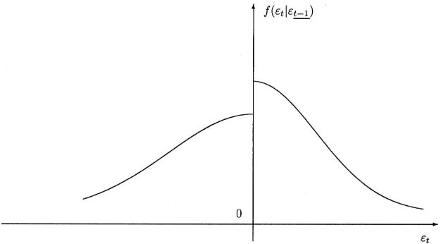
Fig. 1. Conditional density function ofet.
2.1. Conditional distribution
A"rst step in the direction of modeling the conditional distribution was taken by Hansen (1994), who directly speci"ed it as a function of the information set, depending on a low-dimensional parameter vector. If contemporaneous asym-metry holds, the conditional distributions of e`t and !e~
t are di!erent. The
converse is not necessarily true: a simple example is obtained by taking a semi-strong GARCH with an asymmetric distribution for Z
t. However, in the
classical GARCH frameworkZ
t andet have similar conditional density
func-tions (e.g., normal, unimodal, symmetric, asymmetric, etc.). In the present framework, the conditional distribution ofe
tis a mixture of the distributions of
Z`t andZ~
t , with time-varying mixing coe$cients. Assume, for instance, that the
density function ofMZ
tNis unimodal. Then, graphically, the conditional
distribu-tion ofe
tfor the case ofpt,`(pt,~will be as in Fig. 1. At timet#1 the shape of
the conditional distribution will be di!erent. When the variablesp
t,`andpt,~are nondegenerate, the positive and negative
parts of e
t are of course conditionally heteroskedastic, with conditional
vari-ances given byp2
t,`<(Z`t ) andp2t,~<(Z~t ), respectively. Moreover,
<(e
tDet~1)"p2t,`<(Z`t )#p2t,~<(Z~t )#2pt,`pt,~. (2)
2.2. Heteroskewness,heterokurtosis
In the semi-strong GARCH setting, the conditional skewness and kurtosis of e
Contrariwise, when contemporaneous asymmetry holds, the conditional skewness and kurtosis are time-varying. To quantify this, let us introduce the strong innovation process Mg
tN of MetN, de"ned as gt"et!E(etDet~1)"
tNare easily shown to be, respectively, equal to
s
t and st can be expressed as functions of the ratio
p
t,`/pt,~. When it is equal to one at date t, the conditional skewness and
kurtosis coincide with those of the i.i.d. processMZ
tN. This is in particular the
case, at all dates, when contemporaneous asymmetry does not hold (p
t,`"pt,~). From an empirical point of view, these calculations show that the
concept of contemporaneous asymmetry should allow to reconsider the prob-lem of negative skewness or excess kurtosis arising in"nancial data.
2.3. Autocorrelation structure ofMe`t , e~t N
In this section, we characterize both types of symmetries in terms of the autocorrelation structure of the vectorMe`t , e~
t N.
Contemporaneous symmetry implies that cov(e
t,zt~1)"0, for all variable z
t~13et~1, zt~13¸2. In particular, we have ∀k'0, cov(e
t, e`t~k)"cov(et,e~t~k)"0.
Similarly, we can characterize dynamic symmetry (i.e., absence of the so-called leverage e!ect) by
∀k'0, cov(e`t , et~k)"cov(e~t ,et~k)"0.
In the usual GARCH framework (et"p
tZt), the last condition is equivalent to:
(∀k'0) cov(p
t, et~k)"0, which can also be written as cov(pt, e`t~k)"
cov(p
and negative values ofe
t (for at least one lagk), have di!erent impacts on the
current volatility.
Let us remark that when (at least) one form of symmetry holds, Me
tN has
automatically the autocovariance structure of a white noise. When both types of asymmetries are ruled out,Me`t , e~
t Nis nonautocorrelated.
3. Model speci5cation
In this section, we propose a class of GARCH-type models able to capture the features presented in Section 2. Therefore, we have to parameterizeMp
t,`Nand
Mp
t,~Nas positive functions of theet past values. To accommodate
contempor-aneous asymmetry we need di!erent speci"cations for these variables. More-over, to allow for dynamic asymmetry we have to parameterize Mp
t,`N and
Mp
t,~Nas asymmetric functions of the past positive and negative innovations.
A natural choice, which makes the model very tractable, is to choose them linear in these past positive and negative parts of the noise.
We therefore consider the following model:
e
The model can be written in the equivalent form as
[I!B(¸)]
C
pt,`We make the following assumptions on the lag polynomials:
(A1)I!B(¸) is invertible (i.e., the roots of its determinant lie outside the unit circle);
From (A1), p
t,` and pt,~ can be expressed as linear functions of the past
values ofe`t ande~
t . From (A2),pt,`'0 andpt,~'0. Of course, in empirical
applications, it is simplest (although not equivalent, see Nelson and Cao (1992)) to assume the nonnegativity of each coe$cient in (5) instead of (A2). A crucial consequence of the positivity ofp
t,` andpt,~ is that
e`t "p
t,`Z`t and et~"pt,~Z~t . (7)
This will make possible the analysis of the probability structure of the model. Another important consequence of (7) is to allow for interpretation: p
t,` and
pt,~ are, up to constants, the conditional standard deviations of e`t and e~t , respectively. As a particular case, the class contains the GTARCH model introduced by ZakomKan (1994) in which only dynamic asymmetry holds (by
imposing equal coe$cients in the dynamics ofp
t,`andpt,~). It should be noted
that, apart from the GTARCH case, dynamic asymmetry cannot be straightfor-wardly characterized in terms of the model coe$cients.
It is important to notice that the probabilities of occurrence of positive and negative shocks are independent of the past (since the sign ofe
t is that ofZt).
Moreover, if we assume that the median of the distribution ofMZ
tNis zero, the
probabilities are equal. However, conditionally to the past, the expected magni-tudes of a positive and a negative shock are di!erent. Finally, these expected magnitudes are a function of both the magnitudes and the signs of past positive shocks.
While the functional form of the model is rather complicated it can be useful to focus on the e!ects of news on volatility. A paper by Engle and Ng (1993) put forth the idea of a news impact curve which characterizes the impact of past return shocks on the return volatility. Holding constant the information dated
t!2 and earlier, it consists in examining the implied relation betweene
t~1and
the time-tvolatility. Our model di!ers from the standard GARCH-type models in that it allows for di!erent functional form of the volatilities of positive and negative innovations. Therefore, we will consider the two corresponding news impact curves. In general, both of them have di!erent slopes for their positive and negative parts. In the following example (Fig. 2), we assume that the volatilities of the positive and negative parts ofe
t display inverted asymmetries.
It is seen that an unexpected drop in price at timet!1 (e
t~1(0) increases the
volatility (p
t,~) of a decrease at time t more than an unexpected increase in
price (e
t~1'0) of similar magnitude. Conversely, as far as the volatility
p
t,` of an increase at time t is concerned, an unexpected drop decreases
Fig. 2. News impact curves. The news impact curve ofp
t:"J<(etDet~1) is also plotted in the same"gure.
It should be noted that, the two sides of the curves are nonlinear. From Eq. (2), it is seen that this nonlinearity does not occur when<(Z`
t )"<(Z~t )"1 in which
casep
t"pt,`#pt,~.
4. Stationarity
In this section, we derive su$cient conditions for the existence of weak stationary solutions to model (4), (5), in the lines of Bougerol and Picard (1992).1
We also give su$cient conditions for the existence of white noise solutions.
1Necessary and su$cient conditions for wide-sense and strict stationarity of threshold GARCH models of the form (1) (withj"1) have been established by ZakomKan (1994) in the GARCH(1,1) case.
They have been generalized to higher-order lag polynomials by Gonc7alves and Mendes Lopes (1994,
We need to introduce the following notations. For convenience we can always suppose thatp'1,q'2, by adding some coe$cients equal to zero if needed. For allt3Z, let
X
t"(pt`1,`,pt`1,~,2,pt~p`2,`, pt~p`2,~,e`t ,
!e~
t ,2, e`t~q`2,!e~t~q`2)@3R2(p`q~1)
and
a
`"(a`2,`, a~2,`,2, a~q~1,`)3R2(q~2),
a~"(a`2,~, a~2,~,2, a~q~1,~)3R2(q~2),
a
`(Zt)"(b`1,`#a`1,`Z`t , b~1,`!a~1,`Z~t ,
b`2,`, b~2,
`,2, b`p~1,`,bp~~1,`)3R2(p~1),
a
~(Zt)"(b`1,~#a`1,~Z`t , b~1,~!a~1,~Z~t ,
b`2,~, b~2,~,2, bp`~1,~, b~p~1,~)3R2(p~1),
b
`(Zt)"(Z`t , 0, 0,2, 0)3R2(p~1), b~(Zt)"(0,!Z~t , 0,2, 0)3R2(p~1).
De"ne the 2(p#q!1)]2(p#q!1) matrixC(Z
t), written in block-form, by
C(Z
t)"
A
a
`(Zt) b`p,` b~p,` a` a`q,` a~q,`
a
~(Zt) b`p,~ bp~,~ a~ a`q,~ a~q,~ I
2(p~1) 0 0 0 0 0
b
`(Zt) 0 0 0 0 0
b
~(Zt) 0 0 0 0 0
0 0 0 I
2(q~2) 0 0
B
andb"(a0,`, a0,~, 0,2, 0)@3R2(p`q~1). Then, an equivalent representation of (6) is
X
t`1"C(Zt`1)Xt#b. (8)
SinceMC(Z
t)Nis a sequence of i.i.d. square matrices, withC(Zt`1) independent
of X
t, the multivariate linear stochastic di!erence equation (8) makes MXtN
a Markov process. This is used to establish the stationarity results. We use
o(M)"maxMDall eigenvalues of MDNto denote the spectral radius of a matrix
Theorem 1. LetCI"E[C(Z
t)]andCH"E[C(Zt)?C(Zt)].Then if
max(o(CI ),o(CH))(1,
model (4), (5) has a unique second-order stationary solutionMe
tN. Moreover, the
solution is also strictly stationary and ergodic.
Once the stationarity conditions are ful"lled, the following result is helpful to obtain the autocovariance structure (till lagq) ofMe`t , e~
t N.
Corollary 1. Suppose that the assumptions of Theorem 1 hold. Let =
t"[Vec(XtX@t)@,X@t],bI"[Vec(bb@)@]@,and
AI"
C
CH b?CI #CI?b0 CI
D
.Then we haveE[=
t]"(I!AI )~1bI.
Remark. (a) We have obtained conditions ensuring existence of a solution in ¸2and it was proved that the solution is also strictly stationary. Under less restrictive conditions, the existence of a strictly stationary solution which is not necessarily squared integrable can be established. More precisely, a necessary and su$cient condition for the existence of a (unique) strictly stationary solution is that the top-Lyapunov exponent associated with the matricesMC(Z
t)Nin (8) is
strictly negative (see El Babsiri and ZakomKan, 1997 for more details).
(b) It is worth noting that, contrary to standard GARCH models, the second-order stationary solution to model (4), (5), when existing, is not necessarily a white noise. This is due to the fact that MetN is not a martingale di!erence. However, the model can be constrained to produce a white-noise solution. In a previous draft of the paper, two sets of su$cient conditions were provided, both of them corresponding to a"nite number of constraints on the coe$cients (see El Babsiri and ZakomKan, 1997).
5. Consistency of quasi-maximum-likelihood estimators
(a) the conditional mean is identically zero; or (b) both the assumed and the true innovation densities are symmetric around zero. When these conditions do not hold, they also have shown that an additional location parameter is needed to ensure asymptotic identi"ability.
In this section, we will establish the consistency of two sequences of QMLE under di!erent assumptions. At "rst sight it is tempting to use the theory developed by Newey and Steigerwald (1997). However, rewriting (4) in terms of the conditional mean and variance ofe
t as
t is not in general i.i.d. and independent of the past (we have ut"
(pt,`/pt) (Z`
t !1)#(pt,~/pt) (Z~t #1)). Although our model is not nested in the
framework of Newey and Steigerwald (1997), we will obtain some similarities as far as the identi"cation issue is concerned.
The proof is not limited to the GARCH(1,1) case. The general setup is the following. Let M>
tN be a real ergodic, regular, second-order and strictly
stationary process. The statistical model is an ARMA(P,Q) model of the form
P
roots. In addition, the linear innovation MetN of M>
tN is assumed to be the
solution of model (4), (5).
The parameter vector of the model de"ned by (10), (4), (5) is denoted as h. Now, let>
1,2,>T denote¹ observations of processM>tN, obtained for the
true valueh0. Letdbe a strictly positive constant. The unknown parameterh0
is assumed to belong to the interior of the compact parameter space H d such that, ∀h3H
d: (i) the polynomials Uh(z)"1#+Pi/1hizi,
Wh(z)"1#+P`Qi/P`1h
izi, (resp. det(Ah(z)) and det(I!Bh(z)), see Eq. (11)) have
only zeros outside the disk DzD(1#d and no common roots; (ii) min(h
P`Q`1, hP`Q`2)*d (see (11)); (iii) the polynomials (I!Bh)~1 and Ah have nonnegative coe$cients. For all h3H
d, we consider the sequence
The variablese
t(h), pt,`(h) andpt,~(h) can be approximated, fort"1,2,¹,
by e
t(h), st,`(h) and st,~(h), respectively, obtained using the same recursive
formulas (11) but setting all unknown starting values to zero.
The Gaussian quasi-likelihood function (i.e., corresponding to the assumption thatZ
t is Gaussian (0,1), although we do not need to make this assumption) for
the sample of¹observations is
¸
The QML estimatorhKT is obtained by maximizing¸
T(h). To prove thathKT
is consistent, we need to ensure asymptotic identi"ability of the parameter (i.e., to prove that the true value of the parameter is the unique maximizer of the limit function de"ned as the expected value of the loglikelihood). We "rst show that if either: (i) the innovation in (10) is directly observed; or (ii) the model precludes contemporaneous asymmetry; then the asymptotic identi"cation condition is satis"ed. In this approach, we need no assumption on the moments of the positive and negative parts of the i.i.d. process: we only assume that E(Z
t)"0 and <(Zt)"1. We obtain the following consistency
result.
Theorem 2. Suppose that one of the two following assumptions holds:
(i) p`t (h)"p~t (h) a.s. ∀h3H
In the general case, asymptotic identi"ability requires a modi"cation of the quasi-likelihood function. Although theu
t's in (9) are not i.i.d. nor conditionally
Gaussian when p`t Op~
2However, because the measure of the parameter set where the nondi!erentiability occurs is equal to zero, the problem does not arise in practical applications.
assumption. Therefore, we set
¸I
T(h)"
1 ¹
T
+
t/1
lI
t(h), (13)
where
lI
t(h)"!
A
logst(h)#(e
t(h)!st,`(h)#st,~(h))2
2s2
t(h)
B
where
s
t(h)2"s2t,`(h)<(Z`t )#s2t,~(h)<(Z~t )#2st,`(h)st,~(h).
LethIK
T denote the modi"ed QML estimator obtained by maximizing ¸IT(h).
The next result shows thathIK
T is consistent under additional moment
assump-tions on the i.i.d. processMZ
tN. Here we need to be more speci"c concerning the
"rst two moments of the vectorMZ`t ,Z~t N.
Theorem 3. Suppose that the variances ofZ`t andZ~t are known. Then,
hI K
TPh0 a.s. as ¹PR.
From the proof of the theorem, the assumption that the variances of the positive and negative parts of (Z
t) equal to 1, is necessary to ensure thath0 is
the unique maximum of the asymptotic criterion. Otherwise, h0 is indeed a maximum but uniqueness is not guaranteed.
Once consistency of the estimator has been proved, the next step is obviously to establish su$cient conditions for its asymptotic normality. However, this is substantially more di$cult and left for future work. Indeed, the behaviour of the loglikelihood is far from being standard since it is in general not even continuous in the conditional mean parameters (although there is only a countable set of discontinuity points). In the case of lack of contemporaneous asymmetry (condi-tion (i) in Theorem 2), the loglikelihood is continuous but remains nondi!erenti-able for certain values of the conditional mean parameters (such thate
t"0).2
Therefore, some elaborate techniques for proving asymptotic normality, such as Huber's (1967), seem to be required.
6. Empirical application to the French stock index
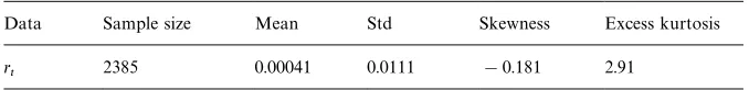
Table 1
Summary statistics of the compounded returnr t
Data Sample size Mean Std Skewness Excess kurtosis r
t 2385 0.00041 0.0111 !0.181 2.91
number of empirical studies based on GARCH-type models. For instance, Glosten et al. (1993), Rabemananjara and ZakomKan (1993), ZakomKan (1994) found
evidence of asymmetries in the volatility of American and French stock Returns. However, for the latter returns, Black's intuition was far from being fully supported by the data. It was shown that: (i) the relative impacts of negative and positive shocks on the current volatility are not the same at all lags; (ii) small shocks and large shocks can provide inverted asymmetries. Our aim in this section is to"nd empirical evidence for the introduction of di!erent dynamics for positive and negative shocks.
The data consist of a series of a daily stock index: the French CAC 40, which is a value-weighted index computed from 40 stocks traded on the monthly Settle-ment Market. It is built to represent the whole range of equities listed on the Paris Bourse and it is used in futures and options markets. The data cover the period from 3 November 1988 to 3 November 1998 involving 2485 observations. However, we used only 2385 observations to estimate the models, keeping 100 observations for out-of-sample comparisons.
DenoteS
t as the price index andrt"logSt!logSt~1 as the compounded
return at time t. In Table 1, some summary statistics for r
t are reported. We
can see that the series is negatively skewed, so large negative returns are more common than large positive ones. Moreover, the excess kurtosis forr
t indicates the existence of a characteristic fat-tailed behaviour compared
with a normal distribution. The Jarque and Bera (1980) normality test statistic is far beyond the critical value which suggests that r
t is far from a normal
distribution.
Before the general model is"tted to the data, its underlying assumptions have to be veri"ed empirically. The main point is the occurrence of asymmetries in the conditional distributions. Recall that, from Section 2.3, symmetries of both types are characterized by very simple moment conditions. Table 2 allows for a precise description of the autocorrelation structure ofr
t, DrtD, (r`t ,r~t ) for lags 1}5 and
obtained for absolute or squared returns. In e!ect, the autocorrelations of the absolute values appear highly signi"cant, which implies rejection of indepen-dence. The autocorrelation structure of (r`t ,r~
t ) is much more informative since
it shows that both asymmetries are contained in the data. Although it is not a formal test, comparing lines 3 and 5 (or 4 and 6) in Table 2 reveals that the leverage e!ect is present, while contemporaneous asymmetry results from the fact that lines 5 and 6 are not similar.
6.1. Estimation of asymmetric GARCH models
To catch these empirical features, several GARCH-type models are"tted to the data. In accordance with many empirical studies and from a preliminary analysis, an AR(1) model is selected for the mean equation. To model the conditional variance, we limit ourselves to GARCH (1, 1)-type models, i.e., low-order speci"cations. This choice is obviously motived by parsimonious reasons and also by the fact that it seems su$cient to highlight the di!erent features taken into account by the models. The BHHH algorithm is used to maximize the likelihood functions. In the "rst three cases, we assume that
e
t"WeptZ"rst estimate a symmetric volatility structure in which, following thet with (Zt) i.i.d.N(0, 1).
argument of Davidian and Carroll (1987) developed in the i.i.d. case, volatility is modeled via absolute values. The estimated model (Model I in the sequel) is as follows, with estimated asymptotic standard errors given in parentheses under estimates:
r
t"0.00046 #0.0218 rt~1 # et,
(0.00001) (0.0001)
p
t"0.00127#0.143 Det~1D#0.777pt~1.
(0.00010) (0.000) (0.000)
We then introduce dynamic asymmetry in the volatility structure. The follow-ing results (Model II) are obtained:
r
t"0.00051 #0.0255 rt~1#et,
(0.00010) (0.0003)
p
t"0.00114 #0.091 e`t~1!0.216e~t~1#0.782pt~1.
(0.00010) (0.002) (0.003) (0.003)
In both models, the estimates are obtained without constraining the para-meters. The results are in accordance with those provided by Rabemananjara and ZakomKan (1993) in a shorter period. The main feature is the evidence of
Table 2
Sample autocorrelation functions ofr
t,DrtDand (r`t,r~t)
Autocorrelation at lagk 1 2 3 4 5 10 20 40
o(r
t,rt~k) 0.030 0.005 !0.032 0.028 !0.046! 0.016 0.003 !0.019 o(Dr
tD,Drt~kD) 0.090! 0.100! 0.118! 0.099! 0.086! 0.118! 0.055! 0.032 o(r`t,r`t~k) 0.037 !0.006 !0.013 0.029 !0.039! 0.017 0.023 0.001
o(!r~t,r`t~k) !0.013 !0.035 !0.019 !0.025 !0.028 !0.007 !0.020 0.017
o(r`t,!r~t~k) 0.026 0.088! 0.135! 0.047! 0.088! 0.056! 0.049! 0.065!
o(r~t,r~t~k) 0.060! 0.074! 0.041! 0.070! 0.027 0.077! 0.015 !0.008!
!Indicate parameters which are statistically signi"cant at the 5% level.
El
Babsiri,
J.-M.
Zakoian
/
Journal
of
Econometrics
101
(2001)
257
}
294
have been performed using the estimates of the covariance matrix of the parameters). As noted by many authors (see, e.g., Nelson, 1991; Ding et al., 1995), volatility tends to rise in response to excess returns lower than expected and to fall when the converse is true.
Contemporaneous asymmetry is tested by allowing two di!erent volatilities for each component of the noise, keeping a symmetric structure for the volatil-ities. The estimation results (Model III) are as follows:
r
t"0.00035 #0.0252 rt~1#et,
(0.00001) (0.0011)
pt,`"0.0007 #0.115 Det~1D#0.426 (pt~1,`#p
t~1,~),
(0.0001) (0.040) (0.007)
p
t,~"0.0012#0.118Det~1D#0.399 (pt~1,`#pt~1,~).
(0.0004) (0.062) (0.007)
All the coe$cients in the volatilities equations are signi"cantly positive. The Wald tests fail to detect di!erences between the coe$cients of De
t~1D and the
intercepts. Conversely, the estimated volatility coe$cients are signi"cantly dif-ferent from one another.
Finally, the general asymmetric structure is estimated. Here we assume that (4) holds with (Z
t) i.i.d.N(0, 1), and the following model (IV) is obtained:
r
t"0.0006 # 0.0261 rt~1#et,
(0.0001) (0.002)
pt,`"0.00094#0.081e`t~1!0.183et~~1#0.399pt~1,`#0.388 pt~1,~,
(0.00007) (0.004) (0.004) (0.025) (0.005)
p
t,~"0.00354#0.037e`t~1!0.217e~t~1#0.370pt~1,`#0.240 pt~1,~.
(0.00041) (0.002) (0.008) (0.008) (0.038)
To check the stationarity condition, the expectations involved in Theorem 1 are obtained via simulations. The computation of the eigenvalues of the matrices involved in Theorem 1 shows that the estimated model is indeed second-order stationary. All parameters are signi"cant at the 5% level. The estimated coe$-cients indicate that both types of asymmetries are present in the data. Interest-ingly, by comparison with the preceding model, allowing dynamic asymmetry provides a more pronounced contemporaneous asymmetry.
Table 3
Estimated quasi-loglikelihoods, excess kurtosis and MSE!
MODEL loglikelihood i MSE (]10~3)
I: SYMMETRIC 7385.2 2.49 0.245
II: With DYNAMIC ASYMMETRY 7390.6 2.72 0.280
III: With CONTEMP. ASYMMETRY 7396.1 2.57 0.239 IV: With ASYMMETRIES of BOTH TYPES 7415.5 2.44 0.187
!Models I}IV refer to the estimated models of Section 6.1.idenotes the empirical excess kurtosis of the standardized residualse(
t/p(t. For models III and IV,p(tis calculated from (2).
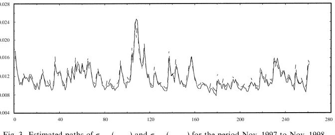
Fig. 3. Estimated paths ofpt,`(**) andpt,~(- - - -) for the period Nov. 1997 to Nov. 1998.
for both asymmetries simultaneously produces a LR test statistic against model II (resp. III), of 24.9 (resp. 19.4) which has an asymptotic p-value of less than 0.001. It is also seen that the general model exhibits less excess kurtosis in the normalized residuals than the other parameterizations. However, we are not able to perform a rigorous test in this framework, and the di!erence might not be signi"cant. Finally, to further compare the di!erent speci"cations, we computed for each estimated model, 100 out-of-sample one-period-ahead predictions. The results are displayed in Table 3. Again, although it is not a formal test, it is seen that our general model outperforms the particular cases. These results provide strong evidence that including both types of asym-metries is statistically important as a description of the time-series properties of "nancial data.
Fig. 3 presents the paths of the estimated volatilities over the last year of the sample. Fig. 4 gives the path of the variable 100(1!pt,`/pt,~) for the same sub-sample. It can be seen that the magnitude of the di!erence (pt,~!p
t,`)
often represents a signi"cant percentage (between 5 and 15%) of p
t,~. The
Fig. 4. Estimated path of 100(1!p
t,`/pt,~) for the period Nov. 1997 to Nov. 1998.
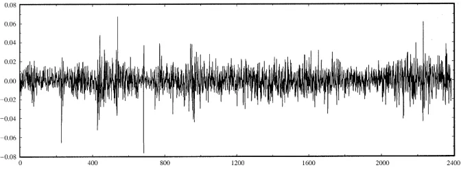
Fig. 5. Estimated residualsetfrom the general asymmetric model of Section 6.1, for the period Nov. 1988 to June 1998.
not been constrained to produce white noise residuals (see Section 5). However, classical diagnostic tests on the estimated residuals show that the hypothesis of white noise is fully supported.
Another view of the properties of the estimated model may be obtained through the analysis of the unconditional and conditional kurtoses. Firstly, we investigated through a Monte-Carlo experiment the term structure of uncondi-tional kurtoses, as the horizon over which returns are computed increases. The experiment involves 120 000 simulations of Model IV with i.i.d. standard Gaus-sian innovationsZ
t. The kurtoses of the cumulative returns log(St/St~k) were
Table 4
Term structure of the unconditional kurtosis in Model IV!
Horizon 1 2 5 10 15 20 30 50 100 120
Kurtosis (sim.) 3.53 3.94 4.08 4.01 3.84 3.73 3.54 3.41 3.14 3.13 Kurtosis (obs.) 5.91 5.88 5.89 5.69 5.49 5.50 5.22 * * *
!The simulated kurtoses are computed using a sample of 120 000 simulations of model IV. The kurtosis at horizonkis obtained for the cumulative returns log(S
t/St~k).
Fig. 6. Estimated conditional excess kurtosis ofetfor the period1197to1198.
of kurtosis are also reported in Table 4 (only for values ofkranging from 1 to 30 because the kurtosis is likely to be poorly estimated for higher lags). It is clear that the simulations imply a much lower excess kurtosis over all horizons then the data set. The model has been simulated under the assumption of a condi-tionally Gaussian distribution, which partly explains the di!erences between the two-term structures. Nevertheless, at least for short horizons, the two-term structures have di!erent shapes: the peak of kurtosis is reached for horizons of around 5 days in the model, whereas the sample kurtoses seem to be decreasing when the horizon increases. It should be noted, however, that the estimates computed over di!erent subsets of the whole sample are highly instable, even for small horizons.
Secondly, the properties of the conditional kurtosis were investigated. Fig. 6 is a plot of the empirical conditional excess kurtosis from the general model against time. The volatilitiespt,`andpt,~have been replaced by their estimated values in (3), and the moments of the (theoretically i.i.d.) normalized residuals
Z
t"e`t /pt,`#e~t /pt,~, have been replaced by their empirical counterparts on
Fig. 7. Parametric (- - - -) and nonparametric (**) estimations of the conditional excess kurtosis ofet(100 observations starting from 25/03/89).
of the conditional excess kurtosis has been computed using the kernel method (see, e.g., Pagan and Schwert (1990) for kernel estimation of conditional vari-ances). The conditional moments ofe4t ande2t were calculated with a Gaussian kernel and di!erent choices of the window width. The results appear to be very sensitive to the choice of the window width. The results reported in Fig. 7 are obtained for a bandwidth proportional to the empirical standard deviation of the data, and they show that the two estimators have close behaviours. Other computations on di!erent subperiods lead to similar conclusions. Therefore, it seems that the parametric model IV used to estimate the"rst two conditional moments of e2
t is an adequate representation of the data. To investigate the
behaviour of the conditional kurtosis as a function of the horizon over which returns are computed, we performed another Monte-Carlo experiment. For horizon 1, and given values ofp
t,` and pt,~, the conditional kurtosis can be
explicitly computed using (3). For horizon 2, the numerator is given by
E[g4t`1Det~1]"+4
k/0
A
4
kBE[pkt`1,`pt`4~1,~k Det~1]c(k, 4!k).
The conditional expectation seems di$cult to obtain in closed form, but it can be evaluated by simulations. This procedure was carried out for all conditional expectations involved in the conditional kurtoses of various horizons. The results presented in Table 5 reveal that the conditional kurtoses are quite sensible to the initial values of the volatilities. When these values are equal, the conditional kurtosis at horizon 1 is that of the standard Gaussian distribution. But for higher horizons, the conditional distributions are leptokurtic, re#ecting the contempor-aneous asymmetry of the model. The dynamic asymmetry shows in the fact that when the initial values are inverted, the results can be very di!erent.
6.2. Empirical evidence of asymmetries in stock returns
Table 5
Conditional kurtosis in model IV!
pt,` pt,~ 1 day 5 days 15 days
0.1 0.1 3.00 3.49 3.46
0.2 0.1 3.44 3.31 3.31
0.1 0.2 3.42 3.72 3.68
0.5 0.1 3.43 3.28 3.28
0.1 0.5 4.42 4.13 4.13
!This table presents the estimated conditional kurtoses at various horizons in Model IV for di!erent initial values ofpt,`andpt,~. The computations involve 10 000 simulations.
Table 6
Number of rejections of the null hypothesis in LR tests at the 5% level, for 42 stocks of the CAC! Null hypothesis Alternative hypothesis
Model II Model III Model IV
Model I 20 34 42
Model II * * 42
Model III * * 37
!Numbers I}IV refer to the models in Table 3. Missing values correspond to models which are not nested.
save space the results are not reported here. They can be found in a previous draft of the paper (see El Babsiri and ZakomKan, 1997). The most outstanding
feature is the evidence of contemporaneous asymmetry in almost all assets, even more pronounced than the usual leverage e!ect. For a global comparison of the four models (Symmetric, with dynamic asymmetry, with contemporaneous asymmetric, with both asymmetries) the normal quasi-likelihoods are used to compute LR statistics. This selection criterion chooses the general asymmetric model for a very large majority of assets (see Table 6). For only "ve stocks, including the leverage e!ect in addition to contemporaneous asymmetry appears unnecessary. The table also con"rms that contemporaneous asymmetry is more important in the data than the classical leverage e!ect. To evaluate how dynamic asymmetry a!ects the two volatility processes as a short term e!ect, it is worthwhile comparing the coe$cients ofe`t~1ande~
t~1. Table 7 summarizes
Table 7
News impact sets for the 42 stocks of the CAC index! No. of items a`1,`"a~
1,` a`1,`'a~1,` a`1,`(a~1,` Total
a`1,~"a~
1,~ 9 8 5 22
a`1,~'a~
1,~ * * * *
a`1,~(a~
1,~ 9 7 4 20
Total 18 15 9 42
!Each cell describes the number of stocks corresponding to a particular case of asymmetry (or symmetry) in the volatility equations (e.g., there are seven stocks such that: (i) positive values of
et~1have bigger impacts onpt,`than negative values of the same magnitude; (ii) the converse is true forpt,~).
feature: it is also symmetric for almost half of the sample but for the other assets the asymmetry can be in both directions. Among these assets, there is a predomi-nance of overreactions to past positive changes (15 assets against nine). These results show that the introduction of contemporaneous asymmetry also allows for reconsidering the leverage e!ect problem.
6.3. Comparison with alternative approaches
It is interesting to compare these results with the alternative models proposed by Hansen (1994). As mentioned in Section 2, these speci"cations have been designed to model non-Gaussian time-varying distributions (instead of asymmetries). The"rst step is to consider a family of density functions, noted
g()Dg, j), generalizing the standard normal. The explicit form is given in Appendix C. The interpretation of g is similar to the degrees of freedom in the Student'st density, whereasj'0 (resp. (0) indicates that the mode of the density is to the left (resp. right) of zero and the variable is skewed to the right (resp. left). Then we estimate a symmetric volatility structure and (omitting the conditional mean equation, which is very similar to those already obtained) we get
pt"0.00105#0.120Det~1D#0.751pt~1.
(0.04190) (0.360) (0.137) (14)
to (14), so we do not report it. The estimations obtained for the time-varying degrees of freedom are presented in Appendix C. The results of the "tting suggest a higher loglikelihood (7524.5) as for our asymmetric model (7415.5). However, it is di$cult to be rigorous in this comparison as the models are not nested, which means that basing the usual likelihood ratio test on asymptotic s2 distributions is not theoretically founded. Moreover, several estimated coe$cients are non signi"cant at any reasonable level. Finally, the MSEs are, respectively, equal to 0.000192 and 0.000172 for the Hansen's models. These results lead to the same conclusions as the log-likelihood comparison.
We also found interesting to compare our formulation with a discretized version of a continuous-time stochastic volatility model with correlated Brownian motions. Maximum likelihood estimation of the model proposed by Heston and Nandi (1999) provides the following results:
r
t"0.0003#0.043p2t#ptZt,
(0.0003) (0.001)
p2
t"0.002#0.769p2t~1#0.022 [Zt~1!1.24pt~1]2,
(0.000) (0.007) (0.000) (0.03)
where (Z
t) is an i.i.d.N(0, 1) process. The existence of a signi"cant coe$cient
forp
t~1in the volatility equation con"rms the presence of dynamic asymmetry
in the data. The estimated log-likelihood is equal to 7395.8, which is similar to the values obtained for Model III. However, because the models are not nested it is di$cult to draw de"nitive conclusions. It should be noted, however, that the Heston and Nandi model is unable to capture the contempora-neous asymmetry property since the term p
tZt in the return equation is a
martingale di!erence.
7. Conclusion
In this paper, we introduced and illustrated a new concept of asymmetry in the dynamics of stock returns. Not only do the signs of past shocks a!ect the current volatility, but also, the impact depends on whether the current excess return is lower or higher than expected. This was achieved by relaxing the classical martingale di!erence assumption on GARCH innovation processes. With this model, we are able to capture some e!ects such as contemporaneous asymmetry, heteroskewness and heterokurtosis. An important feature of the proposed model is that, enlarging the class of GARCH-type models, it keeps their tractability: due to its linearity properties, it allows for Markov representa-tions useful to analyze the probability structure; moreover, the statistical pro-cedures currently used in the GARCH framework (two-stage least squares, QMLE) remain consistent under some identi"ability assumptions. In addition, the empirical study suggested that the underlying assumptions of the model (asymmetry of both types, time-varying conditional skewness and kurtosis) can be strongly supported by"nancial data. Comparison with alternative speci"ca-tions shows that our model dominates formulaspeci"ca-tions that do not allow for heteroskewness, heterokurtosis and asymmetries. Another source of informa-tion concerning the condiinforma-tional variance is of course opinforma-tions data. The model of this paper provides a framework for introducing the di!erent implicit volatilities of calls and puts observed by practitioners. A direction of future research could be to consider these implicit volatilities in order to improve option pricing and hedging.
Acknowledgements
J.-M. Zakoian gratefully acknowledges "nancial support from the HCM program. We would like to thank Adel Grar for providing us with the estima-tion program used in the empirical secestima-tion, and Ali Alami for computaestima-tional assistance. We are also grateful for the helpful comments and suggestions from an associate editor and two referees.
Appendix A. Proofs of the results of Section 4
Proof of Theorem 1. We use a similar approach as in Liu and Brockwell (1988). Let us"rst de"ne the followingR2(p`q~1)-valued stochastic processes:
X
n(t)"
C
0 ifn(0,
b#C(Z
and for alln3Z,
=
n(t)"Xn(t)!Xn~1(t), t3Z.
It is easily seen that for alln'0,X
n(t) and=n(t) are measurable functions of
Z
t,Zt~1,2,Zt~n`1. As a consequence, the two processes are strictly stationary
(for"xedn) and the coupleMX
n(t),=n(t),t3ZNis also strictly stationary.
More-over, from the de"nitions ofX
n(t) and=n(t) we have
=
n(t)"
G
0 ifn(0,
b ifn"0,
C(Z
t)=n~1(t!1) ifn'0.
It is then easy to show, by iterating the preceding relation and from the independence of matricesC(Z
t), that the expectation of=n(t) is"nite. Therefore
we can set for alln3Z:
C
n"E[=n(t)=@n(t)]!E[=n(t)]E[=@n(t)]
"E[C(Z
t)=n~1(t!1)=n@~1(t!1)C@(Zt)]
!E[C(Z
t)=n~1(t!1)]E[=n@~1(t!1)C@(Zt)].
Using the independence betweenZ
t and=n~1(t!1) we then have
VecC
n"CHVecME[=n~1(t!1)=n@~1(t!1)]N
#(CI ?CI) VecME[=
n~1(t!1)]E[=n@~1(t!1)]N
"CHVecC
n~1#[CH#CI?CI]
VecME[=
n~1(t!1)]E[=n@~1(t!1)]N.
Moreover,
VecME[=
n(t)]E[=@n(t)]N"(CI ?CI) VecME[=n~1(t!1)]E[=n@~1(t!1)]N.
Finally, if we set
D
n"[(VecCn)@,(VecME[=n(t)]E[=n@(t)]N)@]@
and
R"
C
CH CH#CI?CI 0 CI?CID
,we haveD
LetDD
nDdenote the sum of the absolute values of all the components ofDn.
From Liu and Brockwell (1988, Proposition 2.1), we have the inequality
DD
nD)const. o(R)n@2 at least for large n, which ensures that the ¸2 norm of
MX
n(t)!Xn~1(t)Ndecreases at a geometric rate. By the Cauchy criterion for the
convergence in¸2, the sequenceMX
n(t)Nconverges in mean square for eacht, to
some limit X
t, say. It is easy to see that the limit process is in fact strictly
stationary and can be expressed in terms of present and past values of theMZ
tN
process (i.e.,MX
tNis causal). Therefore, it is also ergodic.
To prove uniqueness, letXI
t denote another second-order stationary causal
solution of (8) and letd
t"Xt!XI t. We havedt`1"C(Zt`1)dt. Let
CI"
C
VecME(dtd@t)!(Edt)(Ed@t)N VecM(Edt)(Ed@t)N
D
.
From the above discussion we have CI"RCI"lim
n?=RnCI"0, which proves
uniqueness ofMX
tNin¸2.
Finally, MetN is ergodic and (weakly and strictly) stationary as the sum of two components of MX
tN. It is also unique in ¸2since there is a one-to-one
correspondance betweenMX
tNandMetNfor a given MZtNprocess. h
Proof of Corollary 1. From (8) we have
Vec(X
stationary andI!AI is invertible. h
Appendix B. Proofs of the results of Section 5
Proof of Theorem 2. To establish the consistency of the QMLE, it will be useful to introduce the (unobserved) objective function
¸H
obtained by replacing Me
The advantage of using¸H
T(h) instead of¸T(h) is that it is based on stationary
ergodic sequences. The "rst lemma justi"es the approximation of ¸
T(h) by
¸H
T(h). h
Lemma B.1. We have almost surely
lim
Proof. (i) We"rst show that lim
t?=suph|HdDe
t(h)!et(h)D"0.
ForQ"0 the result is obvious. Otherwise, let us introduce the square matrix
B"
A
the nonzero eigenvalues ofBare the inverses of those of the polynomialW(z), the spectral radius ofBis less than (1#d)~1for allh3H
d. Therefore, there exists a positive constantc, independent of h, such thatDDBtDD)ctQ(1#d)~t, ∀t'0, where DD)DD denotes any matrix norm (see Francq and ZakomKan, 1998). The conclusion follows.
(ii) Then we show that
lim
where all missing terms are replaced by zeros. It is clear from (i) that the terms
e`t (h)!e`
t (h) and !e~t (h)#e~t (h) converge uniformly to zero as t goes to
in"nity. Then the conclusion follows from similar argument as in (i) since the inverses of the zeros of the polynomial I!B
(iii) Finally, we have
and the same inequality holds for sup h|HdDv
Both terms on the right-hand side of the previous equation go to zero from (i), (ii) and the fact thate
t()) andet()) are continuous functions, hence bounded, on H
d. This completes the proof. h
We now prove the following identi"ability result.
Lemma B.2. Leth3H
Proof. Let us partition the parameter vector into h@"(h(1){, h(2){), where
(i) First, we have∀h3H
d, ∀t3Z, et(h)"etimpliesh(1)"h(1)0 . Otherwise, one
could"nd a linear combination equal to zero of >
t~1,>t~2,2. This is
impossible from the assumption thatM>
tNis a regular process.
(ii) From the invertibility assumptions on the lag polynomials in (11), for all
h3H
where the sequences (c
i,`(h)), (ci,~(h)), (di,`(h)), (di,~(h)) are absolutely
summ-be written as a function ofe
t~2,et~3,2 . SinceZt~1is independent of the past
The conclusion follows from the fact that the orders of the polynomials
Bh andBh
0 (resp.Ah andAh0) are the same, and thatBh andAh (resp.Bh0 and Ah
0) have no common root.
Asymptotic identi"ability is a consequence of the next lemma.
Lemma B.3. For all h3H
d, let ¸H(h)"Eh0(lHt(h)). Under the assumptions of Theorem 2, ¸H(h)exists and attains a unique maximum ath0.
Proof. (i) We"rst prove that ∀h3H
The assumption on the MA polynomialW
h implies that there exists a se-quence of absolutely summable constants (c
i(h)) such that ∀t3Z,et(h)"
From the de"nition of H
d, it is clear that vHt(h)*d2'0. Therefore,
Suppose that assumption (i) of Theorem 2 holds. ThenvH
t(h)3et~1,∀h3Hd
t) is independent of all past variables it is easily obtained by
WhenD(h)"0, we havevHt(h)"vHt ande
Proof. Following the approach of Francq and ZakomKan (1998), let<
m(h1) denote
t(h1) as m goes to in"nity. Therefore, from Lebesgue's theorem we have
lim
m?=Eh0Sm(t)"¸H(h1).
By Lemma B.3, we can write that
lim sup
Proof. The result is straightforward from Lemmas B.1 and B.4, since
sup
a.s. a neighbourhood<(h
1) such as in Lemma B.5. SinceHd is compact, there
for ¹ large enough. Therefore, the QML estimator almost surely belongs to
<(h
Proof of Theorem 3. Since the proof is very similar to that of Theorem 2, we will not give it to save space. However, we proof that the expected quasi-loglikeli-hood has a unique maximum at the true parameter value. For ease of exposition, we assume that the variances ofZ`andZ~, which are known in this theorem, are both equal to 1. Let
lIH
Proof. (i) By similar arguments as in Lemma B.4 it can be shown that
Moreover, ∀h3H
d, p2t(h)3et~1. Therefore, by taking the expectation
condi-tional to the past:
E
h0
C
(u2t!1)A
1!p2
t
p2
t(h)
BD
"0.
Finally, since∀h3H
d, gt!gt(h)3et~1,p2t(h)3et~1 and since MgtNis a
martin-gale di!erence:
Eh 0
C
2g
t(gt!gt(h))
p2
t(h)
D
"0.
Therefore, we have proved that
∀h3H
d, DI(h))0.
(iii) Now suppose thatDI(h)"0. Then the terms into brackets in (19) is a.s. equal to zero, which proves thatp
t(h)2"p2t, a.s. Therefore
p
t,`(h)#pt,~(h)"pt,`#pt,~, a.s.
Since∀h3H
d,pt,`'0,pt,~'0. Moreover, we have
Eh 0
C
(g
t!gt(h))2
p2
t(h)
D
"0
which implies thatg
t"gt(h), a.s. Finally, we have:et!et(h)"2(pt,`!pt,`(h)).
Now, if we had e
t!et(h)O0, >t~1 could be expressed as a function of >
t~2,>t~3,2 . Therefore, the innovation of >t~1 would be zero which is
excluded sinceM>
tNis a non deterministic process. Therefore,et"et(h) and then
pt,`"p
t,`(h) andpt,~"pt,~(h). Finally, from Lemma B.2,h"h0. Therefore,
the result is proved. h
Appendix C. Alternative conditional distributions used in Section 6
Following Hansen (1994), consider the density function (normalized to have zero mean and unit variance)
g(zDg,j)"
G
bc(1#g~21 (bz`a1~j)2)~(g`1)@2, z(!a/b,bc(1#g~21 (bz`a1`j)2)~(g`1)@2, z*!a/b,
where 2(g(R, !1(j(1, and
a"4jcg!2
g!1, b"J1#3j2!a2, c"
Following Hansen (1994), the following speci"cation was adopted for the time-varying degrees of freedom:
gt"2.1# 27.9 1#exp(!k
t)
,
jt"0.91!exp(!lt) 1#exp(!l
t)
and the following estimations were obtained for the data of Section 6 (with estimated asymptotic standard errors in parentheses)
kt" !2.89 # 0.033 et`~1 # 0.013 e~t~1, (0.42) (1.226) (0.450)
l
t" 2.99 # 0.047 e`t~1 # 0.149 e~t~1.
(0.16) (3.010) (20.31)
References
Arzac, E., Bawa, V.S., 1977. Portfolio choice and equilibrium in capital markets with safety"rst investors. Journal of Financial Economics 4, 277}288.
Bakchi, G., Cao, C., Chen, Z., 1998. Empirical performance of alternative option pricing models. Journal of Finance 52, 2003}2048.
Bawa, V.S., 1978. Safety "rst, stochastic dominance and optimal portfolio choice. Journal of Financial and Quantitative Analysis 13, 255}271.
Black, F., 1976. Studies of stock price volatility changes. Proceedings from the American Statistical Association, Business and Economic Statistics Section, pp. 177}181.
Bollerslev, T.P., 1986. Generalized autoregressive conditional heteroskedasticity. Journal of Econo-metrics 31, 309}328.
Bollerslev, T.P., Engle, R.F., Nelson, D.B., 1994. ARCH models. In: Engle, R.F., McFadden, D.L. (Eds.), Handbook of Econometrics, Vol. 4, pp. 2959}3038 (Chapter 49).
Bollerslev, T.P., Wooldridge, J.M., 1992. Quasi maximum likelihood estimation and inference in dynamic models with time varying covariances. Econometric Reviews 11, 143}172.
Bougerol, P., Picard, N., 1992. Stationarity of GARCH processes and of some nonnegative time series. Journal of Econometrics 52, 115}127.
Campbell, J.Y., Hentschel, L., 1992. No news is good news: an asymmetric model of changing volatility in stock returns. Journal of Financial Economics 31, 281}318.
Christie, A.A., 1982. The stochastic behavior of common stock variances: value, leverage and interest rate e!ects. Journal of Financial Economics 10, 407}432.
Das, S.R., Sundaram, R.K., 1998. Of smiles and smirks: a term-structure perspective. Unpublished manuscript, Department of Finance, Harvard University.
Davidian, M., Carroll, R.J., 1987. Variance function estimation. Journal of the American Statistical Association 82, 1079}1091.
Ding, Z., Granger, C.W.J., Engle, R.F., 1995. A long memory property of stock market returns and a new model. Journal of Empirical Finance 1, 83}106.
El Babsiri, M., ZakomKan, J.M., 1997. Contemporaneous asymmetry in GARCH processes. CREST Discussion Paper 9703.
Engle, R.F., 1982. Autoregressive conditional heteroskedasticity with estimates of the variance of U.K. in#ation. Econometrica 50, 987}1008.
Engle, R.F., Ng, V.K., 1993. Measuring and testing the impact of news on volatility. Journal of Finance 48, 1749}1778.
Francq, C., ZakomKan, J.M., 1998. Estimating linear representations of nonlinear processes. Journal of Statistical Planning and Inference 68, 145}165.
French, K.R., Schwert, G.W., Stambaugh, R.F., 1987. Expected stock returns and volatility. Journal of Financial Economics 19, 3}29.
Glosten, L.R., Jaganathan, R., Runkle, D., 1993. On the relation between the expected values and the volatility of the nominal excess return on stocks. Journal of Finance 48, 1779}1801.
Gonc7alves, E., Mendes Lopes, N., 1996. Stationarity of GTARCH processes. Statistics 28, 171}178.
Gonc7alves, E., Mendes Lopes, N., 1994. The generalized threshold ARCH model: wide sense
stationarity and asymptotic normality of the temporal aggregate. Publications de l'Institut Statistique de l'UniversiteH de Paris 2, 19}35.
GourieHroux, C., 1997. ARCH Models and Financial Applications. Springer, New York.
Hansen, B.E., 1994. Autoregressive conditional density estimation. International Economic Review 35, 705}730.
HaKrdle, W., Hafner, C., 2000. Discrete time option pricing with#exible volatility estimation. Finance and Stochastics 4, 189}207.
Hentschel, L., 1995. All in the family. Nesting symmetric and asymmetric GARCH models. Journal of Financial Economics 39, 71}104.
Heston, S.L., Nandi, S., 1999. A closed-form GARCH option pricing model. Preprint.
Higgins, M.L., Bera, A.K., 1992. A class of nonlinear ARCH models. International Economic Review 33, 137}158.
Huber, J., 1967. The behavior of maximum likelihood estimates under nonstandard conditions. Proceedings of the Fifth Berkeley Symposium on Mathematical Statistics and Probability, Vol. 1. University of California, Berkeley, CA.
Jansen, D., Koedijk, K., de Vries, C., 1998. Portfolio selection with limited downside risk. Mimeo Maastricht University.
Jarque, C.M., Bera, A.K., 1980. E$cient tests for normality, homoscedasticity and serial indepen-dance of regression residuals. Economics Letters 9, 153}160.
Jeantheau, T., 1998. Strong consistency of estimators for multivariate ARCH models. Econometric Theory 14, 70}86.
Kallsen, J., Taqqu, M., 1998. Option pricing in ARCH-type models. Mathematical Finance 8, 13}26.
Lee, S.W., Hansen, B.E., 1994. Asymptotic theory for the GARCH(1,1) quasi-maximum likelihood estimator. Econometric Theory 10, 29}58.
Liu, J., Brockwell, P.J., 1988. On the general bilinear time series model. Journal of Applied Probability 25, 553}564.
Liu, J., Li, W.K., Li, C.W., 1997. On a threshold autoregression with conditional heteroskedastic variances. Journal of Statistical Planning and Inference 62, 279}300.
Lumsdaine, R.L., 1996. Consistency and asymptotic normality of the quasi-maximum likelihood estimator in IGARCH(1,1) and covariance stationary GARCH(1,1) models. Econometrica 64, 575}596.
Nelson, D.B., 1990. ARCH models as di!usion approximations. Journal of Econometrics 45, 7}38. Nelson, D.B., 1991. Conditional heteroskedasticity in asset returns: a new approach. Econometrica
59, 347}370.
Newey, W.K., Steigerwald, D.G., 1997. Asymptotic bias for quasi-maximum likelihood estimators in conditional heteroskedasticity models. Econometrica 65 (3), 587}599.
Nijman, T., Sentana, E., 1996. Marginalization and contemporaneous aggregation in multivariate GARCH processes. Journal of Econometrics 71, 71}87.
Pagan, A.R., Schwert, G.W., 1990. Alternative models for conditional stock volatility. Journal of Econometrics 45, 267}290.
Rabemananjara, R., ZakomKan, J.M., 1993. Threshold ARCH models and asymmetries in volatility. Journal of Applied Econometrics 8, 31}49.
Schwert, G.W., 1989. Why does stock market volatility change over time? Journal of Finance 44, 1115}1154.
Schwert, G.W., 1990. Stock volatility and the crash of'87. Review of Financial Studies 3, 77}102. Sentana, E., 1995. Quadratic ARCH models. Review of Economic Studies 62, 639}661.
Taylor, S., 1986. Modelling Financial Time Series. Wiley, New York.
Weiss, A.A., 1986. Asymptotic theory for ARCH models: estimation and testing. Econometric Theory 2, 107}131.
Yamaguchi, K., 1994. Estimating the equity risk premium from downside probability. The Journal of Portfolio Management 20, 17}27.