A model for neural representation of temporal duration
Hiroshi Okamoto
a,c,*, Tomoki Fukai
b,caCorporate Research Laboratories,Fuji Xerox Co.Ltd.,430Sakai,Nakai-machi,Ashigarakami-gun,Kanagawa259-0157,Japan bDepartment of Information-Communication Engineering,Tamagawa Uni
6ersity,Tamagawagakuen6-1-1,Machida, Tokyo194-8610,Japan
cCREST of JST(Japan Science and Technology Corporation),Japan
Abstract
To address how temporal duration is encoded in neural systems, we put forward a simple model for recurrent neural networks. Particular assumptions are only the following two: (1) neuronal bistability and; (2) environmental effects described by a heat bath. The results of Monte Carlo simulation show that population activity triggered at an initial time continues for a prolonged duration, followed by an abrupt self-termination. This time course seems highly suitable for neural representation of temporal duration. The time scale of this prolonged duration is much longer than the time scale of neuronal firing which is of the order of ms. The former time scale implies that of interval timing in cognition and behaviour. Thus, the model provides a possible explanation for a link between these two separated time scales. The Weber law, a hallmark of humans and animals’ interval timing, can also be reproduced in our model. © 2000 Elsevier Science Ireland Ltd. All rights reserved.
Keywords:Neural representation; Temporal duration; Interval timing; Bistability; Random noise; Weber law
www.elsevier.com/locate/biosystems
1. Introduction
That humans and animals are capable of inter-val timing seems obvious as demonstrated by numerous cognitive and behavioural studies. For instance, interval timing between conditioned stimulus and delayed delivery of reward (rein-forcement) is one of the most frequently used experimental paradigms for these studies (Gibbon and Balsam, 1981).
Interval timing involves several processes such as detection, storage or recall of temporal dura-tion. Undoubtedly neural coding of temporal du-ration in some way must be working underlying these processes. Then, how is temporal duration encoded in neural systems?
Despite that several lines of experimental stud-ies have already been conducted to address neural mechanisms of interval timing (for example, see Niki and Watanabe, 1979; Buonomano et al., 1997; Schultz et al., 1997; Chang et al., 1999), we still have little evidence decisive for concluding. A number of hypothetical models have been pro-posed up to now (for review, see Ivry 1996; Miall, 1996). As reviewed by Ivry (1996), they can be
* Corresponding author. Tel.: +81-465-802015.
E-mail address: [email protected] (H. Okamoto)
classified into two categories: clock-counter mod-els and interval modmod-els.
In clock-counter models, outputs generated by a pacemaker accumulate in a task-specific coun-ter. The number of outputs accumulated in the counter represents temporal duration. The scalar expectancy theory (SET), which is a dominant hypothesis in cognitive and behavioural studies of interval timing, belongs to this category, (Gibbon 1971, 1972, 1977; Gibbon and Church 1981; Church and Gibbon, 1982; Gibbon and Church 1984; Gibbon et al., 1984). The model recently proposed by Bugmann (1998), which utilizes dwindling but not accumulating, is considered to be a modified version of a clock-counter model.
In interval models, different time intervals are represented by distinct elements or by different combinations of distinct elements, each element or combination corresponding to a specific interval. There are a variety of models considered belong-ing to this category (for example, Sutton and Barto, 1981; Tank and Hopfield, 1987; Grossberg and Schmajuk, 1989; Miall, 1989; Church and Broadbent, 1990a,b; Ivry, 1996; Montague et al., 1996; Staddon and Higa, 1999).
Several augments have been raised against clock-counter models (see Ivry 1996; Staddon and Higa, 1999). The main objection is that naı¨ve versions of clock-counter models are incompatible with the Weber law, a hallmark of humans and animals’ interval timing (for the Weber law, see Section 2.1). It should, however, be noticed that there is an additional problem that has been overlooked not only by clock-counter models but also by interval models. This refers to the problem of time scale. Time scales characterizing the dy-namics of neuronal firing are of the order of ms, whereas time scales from several hundred ms to several s, sometimes to several min, characterize interval timing in cognition and behaviour. Hence, if we adhere to the doctrine that ‘every-thing can be traced back to neuronal firing’, it becomes necessary to explain a link between these two separated time scales (Miall, 1996). How do time scales much longer than ms emerge from the dynamics characterized by time scales of ms?
In the present study, we put forward a model for neural representation of temporal duration,
which is pacemaker-free as well as providing a possible solution to the problem of time scale. The model also reproduces the Weber law, an experimental hallmark of humans and animals’ interval timing.
2. Theory
2.1. Criterion
We set the criterion that the model should
satisfy three requirements described in the
following.
The most probable neural representation of temporal duration may be as follows: Activity of a population of neurons triggered at an initial time long-lastingly continues, followed by a self-termination at the end of the duration to be represented (Miall, 1996). This view is partly sup-ported by electrophysiological recordings from prefrontal and cingulate cortex during timing be-haviour in the monkey (Niki and Watanabe, 1979). The first requirement is therefore that the model should generate the time course of popula-tion activity as stated above.
The second requirement is that the model should present a possible solution to the problem of time scale.
The third requirement is that the model should reproduce the Weber law, a well-established ex-perimental hallmark of humans and animals’ interval timing. The Weber law states that
the standard deviation s of the distribution
of timed response is a linear function of
the averaged time m; that is, the Weber ratio
s/mis constant with respect to m(see, for review, Gibbon et al., 1997; Bugmann, 1998). The plausibility of the model can therefore be exam-ined by testing whether it can reproduce the We-ber law.
2.2. Model
The model examined by us is extremely simple.
We considered recurrent networks of N neurons
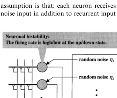
The first assumption is that: Each neuron is bistable if sufficient recurrent input is provided. This means that the firing rate of a neuron is high/low if this neuron is at the up/down state (Fig. 1). It has been proposed in the recent theo-retical study that the voltage dependence of NMDA conductance coupled with GABAergic conductance can generate bistability of the mem-brane potential (Lisman et al., 1998; see also Camperi and Wang, 1998). This may provide possible mechanisms responsible for the neuronal bistability postulated in our model.
The recurrent networks illustrated in Fig. 1 abstract a network structure in some brain region involved in temporal-duration coding, which is presumably located in the prefrontal cortex (Fuster, 1997). In general, each brain region inter-acts with a lot of other brain regions by signal transmissions. The recurrent networks in our model should therefore be considered not as a closed system but as an open system interacting with environments. The simplest but effective way to incorporate the environmental effects is to describe them as a heat bath. Hence the second assumption is that: each neuron receives random noise input in addition to recurrent input (Fig. 1).
2.3. Mathematical formulation of the model
Basically, the time course of the membrane potential of each neuron should be described by the Hodgkin – Huxley equation. However, essen-tial points of our model are the neuronal bistabil-ity and randomness. Without spoiling these essences, we devised to simplify the mathematical formulation. Instead of the Hodgkin – Huxley equation, we used a two-spin Ising system to describe each neuron.
The two-spin Ising system describing the n-th neuron is defined by the Hamiltonian
H(n)
1 or 0;Irepresents recurrent input to this neuron, which is given by
I=GNup
N (2)
with G and Nup being the synaptic strength and
the number of neuron at the up state, respectively. Just for simplicity, the synaptic strength has been set equal everywhere in the networks. IfIsatisfies
u−wBIBu (3)
the system has two stable states: (s1 (n), neuron can be assigned to the former and the down state to the latter. Thus, the description by the two-spin Ising system satisfies the neuronal bistability.
The randomness can also be incorporated into the model if the following stochastic algorithm defines the dynamics of each neuron:
si(n)(t+Dt)=1 with probability pi(n)(t)
This is just the same as the algorithm of the Boltzman machine (Ackley et al., 1985). The time step Dt defines the time scale of neuronal firing. Hence Dt is of the order of ms.
The mathematical formulation of our model is ready in the above. Notice that time scales much
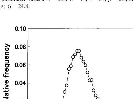
Fig. 2. Time course of population activity P calculated by Monte Carlo simulation according to the stochastic algorithm. The figure shows the results obtained for the following parameter values:N=500; w=10;u=30;b=2.0;Dt=0.002 s;G=24.8.
P=Nup
N (5)
Fig. 2 shows the time course of P obtained by
Monte Carlo simulation according to the stochas-tic algorithm (4). The population activity trig-gered at an initial time is sustained for a prolonged duration, followed by an abrupt self-termination. This is just the desired time course as required in the criterion (see Section 2.1). Notice that the duration is much longer than ms.
Even if all the parameters including the synap-tic strength G are fixed, the duration scatters because of the stochastic nature of the model. Distribution of the duration is shown in Fig. 3, which is obtained by accumulating the results of a large number of trials, each with different random numbers.
The mean duration is a monotonic increasing
function of the synaptic strength G (data not
shown). The mean duration can therefore be adopted to match the duration to be coded by
adjusting G. We further calculated the Weber
ratio (s/m) for differentG’s. The ratio appears to be constant irrespective of m (Fig. 4). Thus, our model can reproduce the Weber law.
Fig. 3. Distribution of the duration of population activity. The distribution was obtained by accumulating results of a number of trials, each with different random numbers. The parameter values used in these trials are the same with Fig. 2.
Fig. 4. Reproduction of the Weber law. For each of the different values ofG, the mean (m) and the standard deviation (s) of the duration of population activity were calculated by sampling 500 trials, each performed with different random number. The results show that the Weber ratio (s/m) is constant withm. The parameter values used in these calcula-tions are the same with Fig. 2 except forG.
longer than ms are not explicitly postulated in this formulation.
3. Results
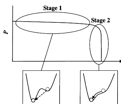
Fig. 5. Schematic description of the mechanisms responsible for the emergence of prolonged time scales from the dynamics characterized by much shorter time scales. For detailed de-scription, see the text.
Since bistability of each neuron is sustained by recurrent input (see the condition (3)), bistability
becomes dulled as I decreases. Finally, at the
point where Icrosses the value u−w, the poten-tial becomes monostable. Just then, all remaining up-state neurons transit to down state by gradient descent. This is just analogous to first-order phase transition in statistical physics.
Escape of neurons from the up to down states with the help of random noise (stage 1 in Fig. 5) proceeds asynchronously and very slowly. In con-trast, transition of the remaining neurons from the up to down states by gradient descent (stage 2 in Fig. 5) happens almost synchronously and very quickly. These are the reason for the emergence of the time course of population activity like that shown in Fig. 2 with prolonged time scales much longer than ms.
Randomness is thus crucial in our model. In previous models, in contrast, randomness was not essential for temporal-duration coding itself but merely added in order to introduce a stochastic nature and to examine their reproducibility of the Weber law (Gibbon, 1977, 1981; Gibbon and Church, 1984; Church and Broadbent, 1990a,b; Allan and Gibbon, 1991; Gibbon, 1992; Gibbon et al., 1997). Our model clears the criterion posed in Section 2.1 with fewer assumptions.
Acknowledgements
The present work has been supported by CREST of JST (Japan Science and Technology Corporation).
References
Ackley, D.H., Hinton, G.E., Sejnowski, T.J., 1985. A learning algorithm for Boltzmann machines. Cogn. Sci. 9, 147 – 169. Allan, L.G., Gibbon, J., 1991. Human bisection at the
geomet-ric mean. Learn. Motiv. 22, 39 – 58.
Bugmann, G., 1998. Towards a neural model of timing. BioSystems 48, 11 – 19.
Buonomano, D.V., Hickmott, P.W., Merzenich, M.M., 1997. Context-sensitive synaptic plasticity and temporal-to-spa-tial transformations in hippocampal slices. Proc. Natl. Acad. Sci. USA 94, 10403 – 10408.
4. Summary and discussion
A model for recurrent networks of bistable neurons, each with random noise input, was ex-amined to address possible mechanisms for neural coding of temporal duration. We have obtained the time course of population activity, which is quite suitable for neural representation of tempo-ral duration (Fig. 2). The Weber law, a hallmark of humans and animals’ interval timing, is also reproduced in our model, which confirms the plausibility of our model.
Camperi, M., Wang, X.-J., 1998. A model of visuospatial working memory in prefrontal cortex: recurrent network and cellular bistability. J. Comp. Neurosci. 5, 383 – 405. Chang, J.Y., Chen, L., Woodward, D.J., 1999. Neural
re-sponses in the fontal cortical, and hippocampal circuits during timing behaviors in freely moving rats. Society for Neuroscience Abstract Vol. 25.
Church, R.M., Broadbent, H.A., 1990a. A connectionist model of timing. In: Commons, M.L., Grossberg, S., Staddon, J.E.R. (Eds.), Quantitative Models of Behaviour: Neural Networks and Conditioning. Lawrence Erlbaum Associ-ates, Hillsdale, pp. 225 – 240.
Church, R.M., Broadbent, H.A., 1990b. Alternative represen-tations of time, number and rate. Cognition 37, 55 – 81. Church, R.M., Gibbon, J., 1982. Temporal generalization. J.
Exp. Psychol. Anim. Behav. Process 8, 165 – 186. Fuster, J.M., 1997. The Prefrontal Cortex, Third Edition.
Raven Press, New York.
Gibbon, J., 1971. Scalar timing and semi-Markov chains in free-operant avoidance. J. Math. Psychol. 8, 109 – 138. Gibbon, J., 1972. Timing and discriminations of shock density
in avoidance. Psychol. Rev. 79, 68 – 92.
Gibbon, J., 1977. Scalar expectancy theory and Weber’s law in animal timing. Psychol. Rev. 84, 279 – 325.
Gibbon, J., 1981. On the form and location of the psychometric bisection function for time. J. Math. Psychol. 24, 58 – 87. Gibbon, J., 1992. Ubiquity of scalar timing with a Poisson
clock. J. Math. Psychol. 36, 283 – 293.
Gibbon, J., Church, R.M., 1981. Time left: linear versus logarithmic subjective time. J. Exp. Psychol. Anim. Behav. Process 7, 87 – 108.
Gibbon, J., Church, R.M., 1984. Source of variance in an information processing theory of timing. In: Roitblat, H.L., Bever, T.G., Terrace, H.S. (Eds.), Animal Cognition. Lawrence Erlbaum Associates, Hillsdale, pp. 465 – 488. Gibbon, J., Church, R.M., Meck, W.H., 1984. Scalar timing in
memory. In: Gibbon, J., Alla, L.G. (Eds.), Annals of the New York Academy of Science: Timing and time percep-tion, vol. 423. New York Academy of Science, New York, pp. 52 – 77.
Gibbon, J., Balsam, P., 1981. Spreading association in time. In: Locurto, C.M., Terrace, H.S., Gibbon, J. (Eds.), Au-toshaping and Conditioning Theory. Academic Press, New York, pp. 219 – 253.
Gibbon, J., Malapani, C., Dale, C.L., Gallistel, C.R., 1997. Towards a neurobiology of temporal cognition: advances and challenges. Curr. Opin. Neurobiol. 7, 170 – 184. Grossberg, S., Schmajuk, N.A., 1989. Neural dynamics of
adaptive timing and temporal discrimination during asso-ciative learning. Neural Networks 2, 79 – 102.
Ivry, R.B., 1996. The representation of temporal information in perception and motor control. Curr. Opin. Neurobiol. 6, 851 – 857.
Lisman, J.E., Fellous, J.M., Wang, X.J., 1998. A role for NMDA-receptor channels in working memory. Nat. Neurosci. 1, 273 – 275.
Miall, C., 1989. The storage of time intervals using oscillat-ing neurons. Neural Comp. 1, 359 – 371.
Miall, C., 1996. Models of Neural Timing. In: Pastor, M.A., Atrieda, J. (Eds.), Time, Internal Clocks and Move-ments. Elsevier Science, Amsterdam, pp. 69 – 94.
Montague, P.R., Dayan, P., Sejnowski, T.J., 1996. A frame-work for mesencephalic dopamine systems based on pre-dictive Hebbian learnng. J. Neurosci. 16, 1936 – 1947. Niki, H., Watanabe, M., 1979. Prefrontal and cingulate unit
activity during timing behavior in the monkey. Brain Res. 171, 213 – 224.
Schultz, W., Dayan, P., Montague, P.R., 1997. A neural substrate of prediction and reward. Science 275, 1593 – 1599.
Staddon, J.E.R., Higa, J.J., 1999. Time and memory: to-wards a pacemaker-free theory of interval timing. J. Exp. Anal. Behav. 71, 215 – 251.
Sutton, R.S., Barto, A.G., 1981. Toward a modern theory of adaptive networks: expectation and prediction. Psy-chol. Rev. 88, 135 – 170.
Tank, D.W., Hopfield, J.J., 1987. Neural computation by concentrating information in time. Proc. Natl. Acad. Sci. USA 84, 1896 – 1900.