AN ACCURACY ASSESSMENT OF GEOREFERENCED POINT CLOUDS PRODUCED
VIA MULTI-VIEW STEREO TECHNIQUES APPLIED TO IMAGERY ACQUIRED VIA
UNMANNED AERIAL VEHICLE
Steve Harwin and Arko Lucieer
School of Geography and Environmental Studies University of Tasmania
Private Bag 76, Hobart, Australia 7001 [email protected]
KEY WORDS:Point Cloud, Accuracy, Reference Data, Surface, Georeferencing, Bundle, Reconstruction, Photogrammetry
ABSTRACT:
Low-cost Unmanned Aerial Vehicles (UAVs) are becoming viable environmental remote sensing tools. Sensor and battery technology is expanding the data capture opportunities. The UAV, as a close range remote sensing platform, can capture high resolution photog-raphy on-demand. This imagery can be used to produce dense point clouds using multi-view stereopsis techniques (MVS) combining computer vision and photogrammetry. This study examines point clouds produced using MVS techniques applied to UAV and terrestrial photography. A multi-rotor micro UAV acquired aerial imagery from a altitude of approximately 30-40 m. The point clouds produced are extremely dense (<1-3 cm point spacing) and provide a detailed record of the surface in the study area, a 70 m section of sheltered coastline in southeast Tasmania. Areas with little surface texture were not well captured, similarly, areas with complex geometry such as grass tussocks and woody scrub were not well mapped. The process fails to penetrate vegetation, but extracts very detailed terrain in unvegetated areas. Initially the point clouds are in an arbitrary coordinate system and need to be georeferenced. A Helmert transfor-mation is applied based on matching ground control points (GCPs) identified in the point clouds to GCPs surveying with differential GPS. These point clouds can be used, alongside laser scanning and more traditional techniques, to provide very detailed and precise representations of a range of landscapes at key moments. There are many potential applications for the UAV-MVS technique, including coastal erosion and accretion monitoring, mine surveying and other environmental monitoring applications. For the generated point clouds to be used in spatial applications they need to be converted to surface models that reduce dataset size without loosing too much detail. Triangulated meshes are one option, another is Poisson Surface Reconstruction. This latter option makes use of point normal data and produces a surface representation at greater detail than previously obtainable. This study will visualise and compare the two surface representations by comparing clouds created from terrestrial MVS (T-MVS) and UAV-MVS.
1 INTRODUCTION
Terrain and Earth surface representations were traditionally de-rived from imagery using analogue photogrammetric techniques that produced contours and topological maps from stereo pairs. Digital photogrammetry has sought ways to automate the process and improve efficiency. Modern mesh or grid based representa-tions provide relatively efficient storage of terrain data at a wide range of resolutions. The quality of these representations is de-pendent on the techniques used for data capture and processing. The representation improves with resolution and the data capture technique must be able to accurately determine height points at sufficient density to portray the shape of the surface. The diffi-culty faced is that the storage and visualisation become increas-ingly difficult as resolution increases. The surface must there-fore be represented by an approximation that resembles reality as closely as possible.
In recent decades photogrammetric techniques have sought to im-prove surface representation through automated feature extrac-tion and matching. Computer vision uses Structure from Mo-tion (SfM) to achieve similar outputs. SfM incorporates view stereopsis (MVS) techniques that match features in multi-ple views of a scene and derive 3D model coordinates and cam-era position and orientation. The Scale Invariant Feature Trans-form (SIFT) operator (Lowe, 2004) provides a robust description of features in a scene and allows features distinguished in other views to be compared and matched. A bundle adjustment can then be used to derive a set of 3D coordinates of matched features. The point density is proportional to the number of matched fea-tures and untextured surfaces, occlusions, illumination changes
and acquisition geometry can result in fewer matches (Remondino and El-Hakim, 2006). The Bundler software1is an open source tool for performing least squares bundle adjustment (Snavely et al., 2006). To reduce computing overheads imagery is often down sampled. Typically the next stage is to densify the point cloud us-ing MVS techniques, such as the patch-based multi-view stereo software PMVS22. Each point in the resulting cloud has an asso-ciated normal. The point clouds produced from UAV imagery (re-ferred to as UAV-MVS) acquired at 30-50 m flying height above ground level (AGL) have a density of∼1-3 points per cm2. There
can be in excess of 7 million points in a cloud (file size of∼500 Mb).
The point cloud generated can be georeferenced by matching control points in the cloud to surveyed ground control points (GCPs). The resulting accuracy is dependent on the accuracy of the GCP survey or reference datasets and in this case it is approximately 25-40 mm (Harwin and Lucieer, 2012). The accuracy can be im-proved with coregistration to a more accurate base dataset.
To allow these large datasets to be used it is usually necessary to convert them into a more storage efficient data structure so that the data can be used in conventional GIS and 3D visuali-sation software that rely on a surface for texturing rather than a point cloud. Grid based (or Raster) and triangular mesh based data models, such as Digital Surface Models (DSMs) and Trian-gular IrreTrian-gular Networks (TINs), are commonly used. After pro-cessing and classification a Digital Elevation Model (DEM) or a Digital Terrain Model (DTM) representation of the earth’s sur-face, without any vegetation or man-made structures, can be
de-1
http://phototour.cs.washington.edu/bundler/ 2
rived. The process of deriving these surface structures from a set of sample points is traditionally done using computational geom-etry based methods such Delauney triangulation or the Voronoi diagram (Bolitho et al., 2009). The data is assumed to be free from noise and dense enough to allow a realistic surface to be derived (Zhou et al. (2010) in Lim and Haron (2012)). When the point cloud is sparse or noisy the resulting surface is often jagged rather than smooth. The surface reconstruction process interpolates heights between sample points (Bolitho et al., 2009). Each point is considered a moment of height change and between points terrain height change is assumed to be linear or is solved by interpolating a least squares fit. An alternative to computational geometry is function fitting, these approaches define a function for determining a surface at a given location by global and/or lo-cal fitting (Bolitho et al., 2009). Kazhdan et al. (2006) developed a Poisson Surface Reconstruction technique that combines both global and local function fitting expressed as a solution to a Pois-son equation (Bolitho et al., 2009). The PoisPois-son approach uses the orientation of the point normal to create a surface that changes gradient according to the change in point orientation (Figure 1). The algorithm obtains a reconstructed surface with greater detail than previously achievable (Jazayeri et al., 2010).
Figure 1: A TIN versus a Poisson DSM.
This paper evaluates the UAV-MVS generated point cloud and surface representations of a natural land form by qualitatively comparing these to a reference dataset generated using close range terrestrial photography based MVS techniques (T-MVS).
2 METHODS
2.1 Study Area
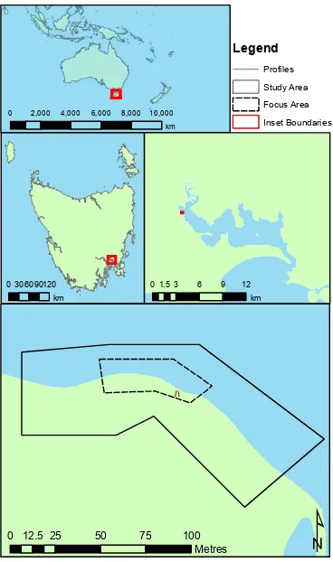
A dynamic 100 m section of sheltered estuarine coastline in south eastern Tasmania will be monitored for fine scale change (Fig-ure 2). The vegetation on the site is grasses and scrub bush along an erosion scarp with salt marsh at the southern end of the study site. For this study a section of the erosion scarp was chosen as the focus area for comparing the close range terrestrial MVS point cloud to the UAV-MVS point cloud (Figure 3).
2.2 Hardware
The camera chosen to capture photography at sufficient resolu-tion for UAV-MVS point cloud generaresolu-tion is the Canon 550D digital SLR camera. This camera has a light weight camera body and provides control over ISO, aperture and shutter speed set-tings. The settings are carefully chosen to reduce motion blur when acquiring images at 1 Hz (one photo per second). The re-sulting image dataset contains around 300 photographs per UAV flight with 70-95% overlap. The OktoKopter micro UAV plat-form (Mikrokopter, 2012) is the basis for the TerraLuma UAV used for this study. The aircraft is an electric multi-rotor system
Legend
Profiles Study Area Focus Area Inset Boundaries
¹
0 2,000 4,000 6,000 8,000 10,000km
0 30 60 90120 km
01.53 6 9 12 km
0 12.5 25 50 75 100 Metres
Figure 2: Coastal monitoring site.
Figure 3: Images of the focus site (the first is taken looking east, the second is taken looking west).
(eight rotors) capable of carrying a∼2.5 kg payload for
mount. This camera is also used for the hand held terrestrial pho-tography. A Leica 1200 real-time kinematic dual-frequency dif-ferential GPS (RTK DGPS) was used to capture ground control.
2.3 Data Collection
To generate the UAV-MVS point cloud 89 photographs were taken from nadir and 64 oblique photographs were taken from a∼45°angle.
The above ground level (AGL) flying height was approximately 30-40 m. Prior to acquiring the UAV imagery 42 small 10 cm orange disks were distributed throughout the focus area. These GCP disks were surveyed using RTK DGPS to an accuracy of
∼1.5-2.5 cm. These disks were placed so that they could be seen
from above and from the waters edge. The UAV imagery cap-tured these GCPs in∼380 overlapping aerial photographs and
then 179 terrestrial photographs were taken of the focus area by hand. The UAV image dataset and the terrestrial dataset were carefully screened and any blurred photographs or photographs beyond the study area were rejected.
2.4 Multi-View Stereopsis
The MVS process relies on matching features in multiple pho-tographs of a subject, in this case a section of coastline. The Bundler software is used to perform a least squares bundle ad-justment on the matched features. These features are discovered and described using invariant descriptor vectors or SIFT feature vectors. Once defined the SIFT features (or in our version SIFT-Fast features3) can be matched and the MVS process produces a sparse 3D point cloud along with the position and orientation of the camera for each image. Radial distortion parameters are also derived. The imagery used in this first step is down sam-pled (5184x3456 pixels⇒2000x1333 pixels). The point cloud produced is in an arbitrary coordinate space. The next stage is to densify the point cloud using PMVS2, usually with down sam-pled images. The improvement made by our UAV-MVS process is that we transform the output from the Bundler bundle adjust-ment so that PMVS2 can run on the full resolution imagery. The resulting set of 3D coordinates also includes point normals, how-ever it is still in an arbitrary coordinate reference frame.
2.5 Georeferencing
The ground control points must identified in the imagery and matched to their GPS positions in the local UTM coordinate sys-tem (GDA94 Zone 55). This “semi-automatic GCP georeferenc-ing” is done by analysing the colour attributes of a random selec-tion of orange GCP disks found in the imagery. The point cloud is then filtered based on the derived colour thresholds, i.e. Red, Green, Blue (RGB) range for GCP orange. The filter finds points in the cloud that are close enough in RGB colour space Euclidean distance to the GCP orange. The extracted orange point cloud contains clusters of points for each GCP and the bounding box of those point clusters is used to calculate a cluster centroid for each GCP cluster in the arbitrary coordinate space. To match these cluster centres to the equivalent surveyed GPS positions, the nav-igation grade on-board GPS positions for the time synchronised camera locations are matched to the Bundler derived camera posi-tions and a Helmert Transformation is derived that, when applied, locates the point cloud in real work scale to an accuracy of∼
5-10 m. The cloud is now in real world scale, therefore the GCP cluster centroid can be matched to the GPS positions by manually finding the closest GCP position to each cluster (when GCPs are more dispersed this process is usually automated). The resulting list of GCP disk cluster centres matched to GCP GPS points is then used to derive new Helmert Transformation parameters for
3
http://sourceforge.net/projects/libsift/
transforming from arbitrary coordinate space to the UTM coordi-nate space.
The terrestrial photography does not have an equivalent set of camera position as the photographs were taken by hand. A “man-ual GCP georeferencing” technique must therefore be under-taken. This involves to extracting and labelling GCP disk cluster centres from the point cloud and then comparing the distribution to the GPS survey. GPS points can then be matched to their asso-ciated cluster centre and a Helmert Transformation can be derived and applied to point clouds and derived surfaces. Once the data was georeferenced it could be clipped into profiles and smaller point clouds using LASTools4.
2.6 Surface Generation
Triangulated meshes join the points in the dataset to their nearest neighbours, for this study the focus is on the points (or vertices) before and after Poisson Surface Reconstruction (since the vertex locations will remain the same when a dense triangulated mesh is created). Poisson surface reconstruction was done using Version 3 of the PoissonRecon software5provided by Michael Kazhdan
and Matthew Bolitho. Default settings were used for all param-eters except octree depth and solver divide, for which the values of 12 and 8, respectively, were chosen based on experimenta-tion. MeshLab6 and Eonfusion7 were used to visualise point
clouds and surfaces and clean the data. Edge face removal using length thresholds were used as well as isolated piece removal (au-tomated and manual). The mesh vertices were then extracted by clipping out the profiles (using LASTools) for comparison with the original MVS derived vertex profiles.
2.7 Point Cloud and Surface Comparison
Future studies will investigate the best methods for quantitatively comparing point clouds and derived surfaces. For this study the method chosen was a qualitative comparison of point cloud pro-files and strips along lines of interest within the focus area (see Figure 4).
Figure 4: The two profiles within the focus area (see Figure 2).
3 RESULTS AND DISCUSSION
The MVS workflow was applied to the terrestrial and the UAV image datasets. For the UAV-MVS dataset, 151 of 153 images chosen were processed resulting in a point cloud ∼175 m by
∼60 m containing∼7.3 million points (∼1-3 points per cm2). For
the T-MVS dataset, 174 of 179 images chosen were processed re-sulting in a point cloud∼175 m by∼60 m containing∼6.3 million
points (∼3-5 points per cm2). Screen shots of these two clouds
and close up views of two 1 m staves are shown in Figure 3.
(a) The UAV-MVS point cloud.
(b) The T-MVS point cloud.
(c) The close up view of the UAV-MVS point cloud (point size = 2).
(d) The close up view of the T-MVS point cloud (point size = 1).
Figure 5: The derived point clouds.
Both point clouds have sparse sections in the woody scrub bush, dead bushes and longer grasses. The UAV-MVS dataset has more points representing vegetation in the central portion of the focus area, this is not surprising due to the occlusion caused by tak-ing the T-MVS photography from the water side of these bushes. Both point clouds have a high density of points on the erosion scarp and for soil and rock in general, even where the scarp is overhanging. The texture of the ground in these areas is ideal for
feature identification as there is a lot of rocky gravel and shell grit in the soil and the beach is very pebbly.
To analyse the effect of surface composition on point density pro-files were visualised and compared. For illustrative purposes a number of screen shots are provided that show regions or views of interest. The Eonfusion scene is a far better viewing environ-ment than the flat screen shots provided as the view perspective can easily be adjusted to focus on interesting features from vari-ous angles.
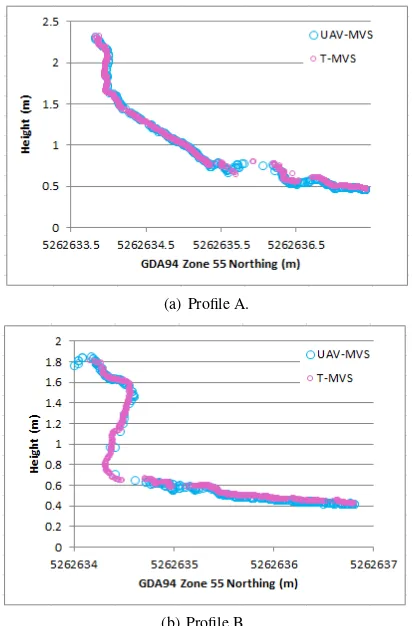
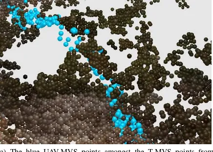
As can be seen in Figure 6(a) and Figure 7(a) showing profile A the blue UAV-MVS points are amongst or slightly below the MVS points. As the profile crosses the vegetation the sparse T-MVS points on the occluded side of the bush can be seen amongst the relatively dense UAV-MVS points.
(a) Profile A.
(b) Profile B.
Figure 6: A 1 cm wide profiles of the UAV-MVS and T-MVS point clouds.
On the pebbly beach the UAV-MVS cloud is consistently below the T-MVS cloud (<1 cm) (see Figure 6(b) and Figure 7(b)). This may simply be due to differences in the Helmert transformation. Coregistration would be required to assess this further in a future study.
The Poisson surfaces derived from these two clouds produced new point clouds of surface vertices. The UAV-MVS Poisson sur-face point cloud (referred to as UAV-MVS Poisson) has 2.3 mil-lion vertices and the T-MVS Poisson surface point clouds (re-ferred to as T-MVS Poisson) has 1.8 million vertices. After clean-ing, the number of vertices were reduced by∼1100 and∼6000
(a) The blue UAV-MVS points amongst the T-MVS points from above.
(b) The blue UAV-MVS points beneath the T-MVS points from below.
Figure 7: A 6 cm wide strip (profile A) of the UAV-MVS point cloud viewed with the T-MVS point cloud.
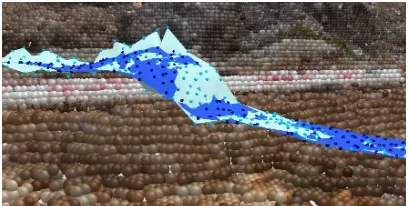
The wider 6 cm profile strips have been created as surfaces to as-sess the difference between UAV-MVS Poisson and T-MVS Pois-son. Figure 3 shows the TIN surface compared to the Poisson surface for T-MVS and UAV-MVS datasets respectively.
In these views the natural coloured point clouds have been offset in the Z dimension by -10 cm to allow visualisation of the shape of the surface compared to the cloud that it was derived from. The surface covers a vegetated section and in the UAV-MVS dataset the denser section previously mentioned can be seen when com-paring this view (Figure 8(a)) to the same view of the shrub (Fig-ure 8(b)). The T-MVS cloud is sparse here and as a result the Poisson surface seems to have exaggerated the shrub height over the sparse section, probably due to the orientation of the normals varying greatly for those few points, which happens in vegeta-tion. The triangulated mesh is much more jagged than the Poisson surface in both views and the UAV-MVS Poisson is particularly smooth (Figure 8(a)). The shrub in reality does have a reasonably smooth shape, in in this instance the UAV-MVS Poisson appears most accurate. To examine this further a section of Profile B that passes through the pebbly beach is visualised. In Figure 9(b) the Poisson surface is again smoother and the drop in terrain at this point point is well represented (see Figure 6(b)). In Figure 9(a) the same seems evident. In Figure 9(c) the Poisson surfaces for UAV-MVS and T-MVS are shown on the T-MVS point cloud (Z-10 cm). In this view the UAV-MVS surface is again∼1 cm below
the T-MVS surface, but the shape of the terrain is basically the same, where as when two raw MVS based TINs are compared in the same view the outliers in the UAV-MVS data seem to cause the surface to vary suddenly causing spikes or peaks in terrain that are not evident in the equivalent T-MVS TIN.
These visualisations provide insight into the quality of terrain and
(a) The UAV-MVS point cloud below Poisson (blue) and TIN (light blue) strips.
(b) The T-MVS point cloud below Poisson (brown) and TIN (pink) strips.
Figure 8: 6 cm wide strips of Poisson and TIN surfaces viewed over a vegetated section of the points clouds from which they were derived (Z-10 cm), each natural coloured dot has a 14mm diameter.
surface extraction possible using MVS techniques. The use of Poisson surface reconstruction has potential advantages over tra-ditional triangulated mesh creation. Poisson surfaces seem gen-erally smoother and smooth surface representations are often bet-ter when undertaking decimation, hydrological analysis, DEM derivative extraction and vegetation and ground filtering. The apparent outliers in the point cloud may not impact on the out-puts from these analyses and, provided the point cloud density is carefully monitored and taken into account when mapping sur-face quality, the result may be more realistic for most sursur-face types. Some vegetated areas have complex geometry (such as complex overlapping branches or tussock grasses) and areas with little or no texture are going to be poorly represented and this may impact on the Poisson reconstruction. The creation of a TIN is still a viable option, particularly when the point cloud can be maintained without decimation. When products with a smaller memory footprint are required there seems to be a strong case for using Poisson surface reconstruction to create a fairly smooth yet detailed representation of the terrain from which lower resolution surfaces can be extracted. The TIN surfaces appear more jagged and these spikes in the terrain can cause erroneous height values in a derived output.
4 CONCLUSIONS AND FUTURE WORK
(a) The UAV-MVS point cloud below Poisson (blue) and TIN (light blue) strips.
(b) The T-MVS point cloud below Poisson (brown) and TIN (pink) strips.
(c) The T-MVS point cloud below UAV-MVS Poisson (blue) and T-MVS Poisson (brown) strips.
Figure 9: 6 cm wide strips of Poisson and TIN surfaces viewed over a pebbly beach section of the points clouds from which they were derived (Z-10 cm), each natural coloured dot has a 14mm diameter.
Two datasets were derived using the technique, one using terres-trial photography and the other using photography acquired via an unmanned aerial vehicle (UAV). The two point clouds provided dense point coverage of the areas captured in the imagery, the ter-restrial MVS dataset had∼3-5 points per cm2and the UAV-MVS
dataset had∼1-3 points per cm2. Once georeferenced the two
clouds coincided quite well, however in future studies compar-ison will be between coregistered datasets. Triangulated mesh-ing and Poisson surface reconstruction was used to create surface models and these models were compared and evaluated to assess how well the terrain and surface features were portrayed. The point clouds produced using MVS have point normals associated with each point and this allows detailed surface features to be de-rived using Poisson surface reconstruction. The derivatives that can be extracted from such a detailed surface representation will benefit from the Poisson algorithm as it combines global and local function fitting and seems to smooth the data and the process is not strongly influenced by outliers in the point cloud. Future stud-ies will undertake quantitative assessment of the differences and evaluate the potential of these techniques for change detection, in this study area the fine scale coastal erosion that is occurring may be indicative of climate change and, if this technique proves useful, UAVs may be a viable tool for focussed monitoring stud-ies. The issues faced in vegetated areas and areas with complex
geometry that result in sparse patches in the point cloud need to be investigated, it may be that the key areas of change are still well represented. The MVS technique has a great deal of poten-tial both in natural and man-made landscapes and there are many potential applications for the use of UAVs for remote sensing data capture, alongside laser scanning and more traditional tech-niques, to provide very detailed and precise representations of a range of landscapes at key moments. Application areas include landform monitoring, mine surveying and other environmental monitoring. Qualitatively, the outputs from the UAV-MVS pro-cess compare very well to the terrestrial MVS results. The UAV can map a greater area faster and from more viewing angles, it is therefore an ideal platform for capturing very high detail 3D snapshots of these environments.
ACKNOWLEDGEMENTS
The authors would like to thank Darren Turner for his logistical, technical and programming support and UAV training. Thank you to Myriax for the scholarship license for the Eonfusion nD spatial analysis package. In addition, for making their algorithms and software available, we would like to give thanks and appre-ciation to Noah Snavely and his team for Bundler, David Lowe for SIFT, the libsift team for SIFTFast, Yasutuka Furukawa and Jean Ponce for their multi-view stereopsis algorithms (PMVS2 and CMVS) and Martin Isenburg for LASTools.
References
Bolitho, M., Kazhdan, M. and Burns, R., 2009. Parallel poisson surface reconstruction. Advances in Visual Computing LNCS 5875, pp. 678–689.
Harwin, S. and Lucieer, A., 2012. Assessing the accuracy of georeferenced point clouds produced via multi-view stereopsis from Unmanned Aerial Vehicle (UAV) imagery. Currently in review, publication pending.
Jazayeri, I., Fraser, C. and Cronk, S., 2010. Automated 3D Object Reconstruction Via Multi-Image Close-Range Photogramme-try. International Archives of Photogrammetry, Remote Sens-ing and Spatial Information Sciences XXXVIII(2000), pp. 3– 8.
Kazhdan, M., Bolitho, M. and Hoppe, H., 2006. Poisson surface reconstruction. In: Proceedings of the Eurographics Sympo-sium on Geometry Processing.
Lim, S. and Haron, H., 2012. Surface reconstruction techniques: a review. Artificial Intelligence Review.
Lowe, D. G., 2004. Distinctive Image Features from Scale-Invariant Keypoints. International Journal of Computer Vision 60(2), pp. 91–110.
Mikrokopter, 2012. ”MikroKopter WiKI”
http://www.mikrokopter.com.
Remondino, F. and El-Hakim, S., 2006. Image-based 3D Mod-elling: A Review. The Photogrammetric Record 21(115), pp. 269–291.
Snavely, N., Seitz, S. M. and Szeliski, R., 2006. Photo Tourism: Exploring image collections in 3D. ACM Transactions on Graphics 25(3), pp. 835.