www.elsevier.comrlocateratmos
Relationship between interdecadal fluctuations in
annual rainfall amount and annual rainfall trend in a
southern mid-latitudes region of Argentina
Omar Abel Lucero
), Norma C. Rodrıquez
´
1( )
Instituto Nacional del Agua y del Ambiente CRS , and National UniÕersity of Cordoba, Pasaje Curupaity´
2460, 5009 Cordoba, Argentina´ Received 21 July 1998; accepted 14 June 1999
Abstract
An amplifying fluctuation is detected in the time series of annual rainfall, starting about
Ž .
mid-1930s in the province of Cordoba central Argentina . The timescale of this fluctuation´ initially had a value approximate to 10 years, and increased to a value of about 20 years. This fluctuation is structured as a train of centers of negative and positive rainfall perturbation alternating in time. A strong positive trend in annual rainfall amount started simultaneously to excitation of amplifying fluctuation. Analyses of contribution from bands of wavelet timescale to reconstruction of time series of perturbation of annual rainfall amount indicate that trend is produced by fluctuations with timescale larger than 10 years. Before 1935, annual rainfall had a stationary mean. After that year, mean annual rainfall in this region is increasing at a rate of 5 mmryear. During the period 1935–1983, the trend produced by contribution from fluctuations with timescale greater than 10 years is 4.6 mmryear. The remaining 0.4 mmryear of trend is produced by fluctuations with timescale smaller than 10 years, and it does not have statistical significance. The amplifying fluctuation in the bands of fluctuations with timescale 10–17 years and 17–27 years, is clearly detected in the 3-month periods November to January, and February to April. These are also the only two 3-month periods with trend statistically significant. Regression analysis of seasonal rainfall on year indicates that there is a discontinuity in trend between the periods 1873–1934 and 1935–1983. In periods November to January and February to April, fluctuations with timescale larger than 10 years produce a statistically significant trend after 1935. Fluctuations with timescale smaller than 10 years do not contribute in a significant way to trend in
Ž .
these seasons. During the 60 years before wave excitation period 1873–1934 , wavelet analysis does not show another amplifying fluctuation of such strong intensity. Finding what triggered this
)Corresponding author. E-mail: [email protected]
1
E-mail: [email protected].
0169-8095r99r$ - see front matterq1999 Elsevier Science B.V. All rights reserved.
Ž .
gargantuan amplifying fluctuation in annual rainfall is an important question for understanding multidecadal climate variability.q1999 Elsevier Science B.V. All rights reserved.
Keywords: Annual rainfall; Argentina; Multidecadal climate variability
1. Introduction
Fluctuations at decadal and interdecadal timescales are ubiquitous phenomena in time series of rainfall and other atmospheric variables. For example, annual rainfall variations
Ž .
with a quasi 20-year period were found by Hu et al. 1998 for central United States ŽMissouri, Illinois, Iowa, Kansas and Nebraska using running-mean analysis and Morlet. wavelet analysis. The same timescale of variability was found for precipitation in the
Ž .
coastal region of central California by Haston and Michelson 1994 . Variability in the 20-year timescale is extended to climate in general as summarized by Trenberth and
Ž .
Hurrel 1994 . Extensive droughts in the central plains of USA in the 1930s and the 1950s were associated to negative rainfall perturbations of a quasi 20-year precipitation
Ž . Ž .
fluctuation as found by Hu et al. 1998 . Latif and Barnett 1996 thoroughly examined the 20-year climatic cycle in the North Pacific and North America. They found evidence that this timescale in climate variability results from coupled oceanic–atmospheric processes.
However, despite their omnipresence, the excitation of decadal and interdecadal fluctuations of atmospheric variables, particularly rainfall, is scarcely documented. Documenting examples of excitation of these fluctuations will provide a clearer picture of their evolution and as well as their relationship with other atmospheric and oceano-graphic variables. Furthermore, the consequence of the excitation of interdecadal fluctuations on the evolution of annual rainfall amount is an unexplored topic.
In this research, we searched for excitation of interdecadal fluctuations in time series of annual rainfall in central Argentina. We found a case of excitation of fluctuation in annual rainfall in the decadal and in the interdecadal timescale. These fluctuations show amplifying intensity. Furthermore, these amplifying decadal and interdecadal fluctua-tions make a decisive contribution to the observed trend in annual rainfall in this region. Description of the characteristics of subdecadal, decadal and interdecadal fluctuations in rainfall amounts and their relationship to a trend in annual rainfall is the purpose of this paper.
Environmental effects of the ascending trend in annual rainfall are notorious in this region in central Argentina. This trend in annual rainfall amounts is bringing about
Ž .
important effects in the hydrologic regime Lucero, 1998a, 1995 . Among these effects,
Ž . Ž .
a large part downtown of Miramar city an important resort area remained inundated by the water of lake Mar Chiquita during the last 25 years. Lake Mar Chiquita is located in northern Cordoba. This persistent inundation led local authorities to demolish that city
´
district in 1991, because it represented a danger to sport yachting, and it affected the scenery of the lake. In some parts of the territory of this province, substantially
Ž .
rainfall amounts result in higher crop yields. This region is a major agricultural area, with state-of-the-art technology; weather effects on crops influence world market prices of several agricultural products.
The organization of this paper is as follows. In Section 2, data set and methods are described. In Section 3, the excitations of amplifying fluctuation at interdecadal timescale, and trend in time series of annual rainfall are described and analyzed. In Section 4 the seasonal variability of amplifying fluctuation and trend in rainfall amount is analyzed. Finally, Section 5 contains the conclusions.
2. Data and method
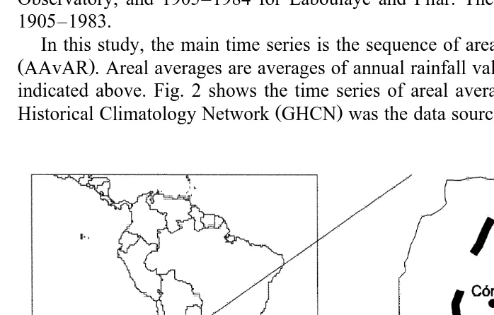
Fig. 1 shows the geographical locations of the rain gauges whose time series of rainfall amount are used in this research. These are Cordoba astronomical observatory,
´
Laboulaye, and Pilar, located in the province of Cordoba. These time series are of
´
excellent quality. Monthly rainfall sequences cover the spans: 1873–1987 for Cordoba
´
Observatory, and 1905–1984 for Laboulaye and Pilar. The main period of analysis is 1905–1983.
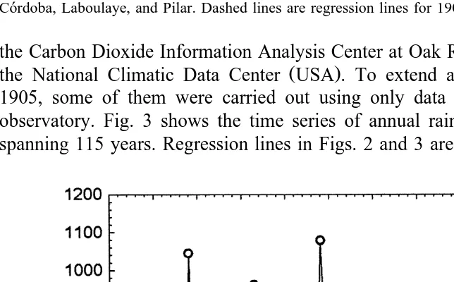
In this study, the main time series is the sequence of areal average of annual rainfall ŽAAvAR . Areal averages are averages of annual rainfall values in the three rain gauges. indicated above. Fig. 2 shows the time series of areal average of AAvAR. The Global
Ž .
Historical Climatology Network GHCN was the data source. GHCN is a joint effort of
Ž .
Ž .
Fig. 2. Time series of AAvAR. Averages calculated using annual rainfall amounts hydrologic year in Cordoba, Laboulaye, and Pilar. Dashed lines are regression lines for 1905–1934, and for 1935–1983.´ the Carbon Dioxide Information Analysis Center at Oak Ridge National Laboratory and
Ž .
the National Climatic Data Center USA . To extend analyses back in time beyond 1905, some of them were carried out using only data from Cordoba’s astronomical
´
observatory. Fig. 3 shows the time series of annual rainfall in Cordoba Observatory,
´
spanning 115 years. Regression lines in Figs. 2 and 3 are described in Section 3.
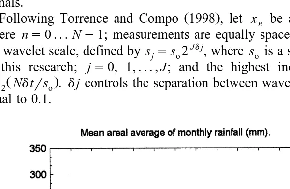
Ž .
This region has a dry season and a rainy season see Fig. 4 . The dry season extends from June to August. The rainy season extends from October to April. Transition months are May and September. Hailstorms and intense convective cells spawning small tornadoes are common in late spring and summer of years with abundant rainfall. In this
Ž
region, the extremes of the Southern Oscillation ENSO and La Nina — Southern
˜
.
Oscillation produce statistically significant effects on monthly rainfall amounts during
Ž .
April, August, November and December Lucero, 1998b . During austral summer, this region is in the southern margin of the monsoon circulation induced by the Bolivian
Ž .
Altiplano Plateau Zhou and Lau, 1998 .
Time-varying components, in time series of annual rainfall, are individualized using the Morlet continuous wavelet transform. Wavelet analysis is increasingly being used in
Ž
atmospheric sciences to analyze time series of several types of variables Meyers et al., .
1993; Weng and Lau, 1994; Mak, 1995; Hu et al., 1998, among others .
Wavelet analysis decomposes the annual rainfall time series into features of similar wavelet timescale; thereby constituent parts can be recognized, and their evolutions can
Ž .
be traced Morlet, 1982; Grossman and Morlet, 1984; Daubechies, 1994; Mallat, 1998 . This aptitude of wavelet analysis is particularly convenient for identifying non-periodic signals.
Ž .
Following Torrence and Compo 1998 , let xn be a time series of rainfall values, where ns0 . . . Ny1; measurements are equally spaced at time interval dt. Let s bej
the wavelet scale, defined by sss 2Jdj
, where s is a starting scale, which is equal 1.8
j o o
in this research; js0, 1, . . . , J; and the highest index J is given by: Jsdjy1
Ž .
log2 Ndtrs .o dj controls the separation between wavelet scales. In this research dj is equal to 0.1.
After wavelet decomposition of the time series of annual rainfall values, x , then
symbols have the following values: c 0 removes a scaling introduced during wavelet
y1r4 w Ž .x transform; its value is equal top . C is a constant with value 0.776. R W sd n j is the real component of the complex wavelet transform. To avoid unnecessary repetition,
Ž .
readers are referred to Torrence and Compo 1998 for further details of the Morlet continuous wavelet transform.
3. Description of decadal and interdecadal fluctuations
3.1. Non-periodic signal analysis of AAÕAR
The time series of AAvAR was scrutinized using wavelets to identify non-periodic components. For each year, the wavelet analysis decomposes the annual rainfall value into contribution from 80 wavelet timescales. Each wavelet timescale makes its own
Ž Ž ..
contribution to the reconstruction of the AAvAR at each year Eq. 1 . The linear correlation coefficient between observed and reconstructed time series of AAvAR is 0.97; they exhibit good agreement; edge effects are small.
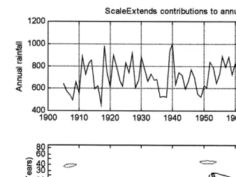
Result of wavelet time–timescale contribution analysis is shown in Fig. 5. This figure Ž . depicts local contribution to annual rainfall perturbation, obtained using Eq. 1 , at
Ž . indicated year and from indicated wavelet period. The annual rainfall perturbation r t
ˆ
Ž . Ž . Ž .
is defined by: r t
ˆ
sr t yr, where r t is the AAvAR, t is year, and r is the mean Žcalculated on the period 1905–1983 of r. r t is reconstructed by summing contribu-.ˆ
Ž .Ž .
tions along a vertical line that is, summing contributions from all wavelet periods . Fig. 5 shows three main features:
Ž .1 Contributions to total rainfall perturbation from bands of wavelet timescale larger than 37 years are small in this region. These bands of wavelet timescales will not be further considered.
Ž .2 Fig. 5 shows that a chirp-like fluctuation is excited in the mid-1930s a chirp-typeŽ
. Ž .
fluctuation has its timescale varying in the band 10 years, 17 years of wavelet timescale; and by late 1950, it expanded to approximately 20-year timescale. Dipole-like structures form this fluctuation. In Fig. 5, a line joins the center of dipoles of this fluctuation. A center of negative rainfall perturbation harbingers the dipole; followed by positive rainfall perturbation. This wavelike fluctuation starts at about 1935 with a leading negative rainfall perturbation. Timing between successive dipoles is approxi-mately coincident with wavelet timescale. The core of negative rainfall perturbation took place in 1935, 1949, and 1969, coincident with severe droughts in the Province of Cordoba. This fluctuation is amplifying since its excitation in the mid-1930s.
´
Ž .3 There are large contributions from a band with wavelet timescales between Ž
approximately 2 years to 8 years. The quasi-biennial fluctuation and ENSO El Nino —
˜
.
Ž .
Fig. 5. Morlet wavelet analysis of the AAvAR. Top: observed time series of AAvAR mm . Bottom: time
Ž
elapsed-timescale representation of the time series of rainfall perturbation annual rainfall values minus mean
. Ž . Ž .
in 1905–1983 . Contours are 0, 5, 10, and 15 solid curves , andy5,y10,y15 dashed curves , in units of millimeters of rainfall at each wavelet timescale. Full line shows the time continuity of the fluctuation excited in the mid-1930s.
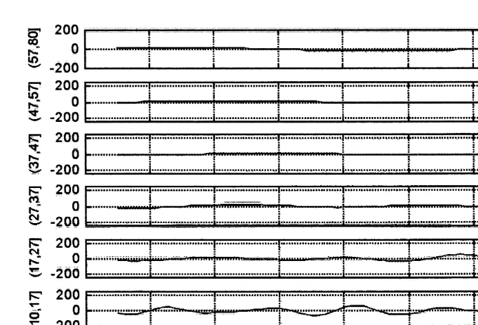
Next, contributions to perturbation of AAvAR were grouped into bands of contribut-ing wavelet timescales. Fig. 6 shows the partial contribution to total rainfall perturbation from each band of wavelet timescales. Largest partial contributions are supplied by bands of wavelet timescale smaller than 27 years. The band of wavelet timescale smaller than 10 years encompasses contributions from timescales similar to the quasi-biennial
Ž .
oscillation, and from ENSO El Nino — Southern Oscillation . The following two
˜
bands, with wavelet timescales centered at 13.5 years and 22 years, includes contribution from the fluctuation excited about mid-1930; these contributions show an amplifying
Ž .
wavelike pattern. In particular, the band of wavelet timescales 17 years, 27 years starts to amplify in mid-1930; then about mid-1950 its amplification rate becomes stronger.
Ž .
The contribution from band 10 years, 17 years amplifies in the mid-1930s, reaches a maximum during the early 1940s, and thereafter dampens until the late 1960s when it starts to amplify again.
Fig. 6. Contribution to perturbation of AAvAR, from indicated bands of wavelet timescales. Y-axes indicate the contribution of band to total annual rainfall perturbation. Bottom panel shows the total perturbation of
Ž .
AAvAR average of three rainfall time series .
Ž . Ž .
timescales 10 years, 17 years and 17 years, 27 years . In contrast, it is seen in Fig. 6 that contribution from band of wavelet timescales smaller than 10 years does not show trend. We proceed next to carry out a regression analysis.
3.2. Trend in annual rainfall during period of fluctuation amplification
Having found an amplifying fluctuation starting in about the mid-1930s in the decadal and bidecadal bands of contribution to the total perturbation of AAvAR, their effects on the evolution of the mean value of AAvAR is examined next. Because the amplifying fluctuation started in about the mid-1930s, we want to know if different patterns of evolution in the AAvAR occurred before and after that time. Fig. 8 shows the time series of 5-year mean of AAvAR, which exhibits two patterns of evolution. The first pattern, before the mid-1930s, lacks a clear trend; the second pattern begins at the time of excitation of the amplifying interdecadal fluctuations. This second pattern shows a positive trend.
Next, using linear regression we analyze the effect of the fluctuations starting in 1935 on the evolution of the mean of AAvAR. The time series of AAvAR was split into two different periods. The first period covers the span 1905–1934. The second period is from 1935–1983. Results indicate that along the period 1905–1934, there was not a statistically significant trend in AAvAR. On the other hand, the period 1935–1983 Žcoincident with the amplifying fluctuations at interdecadal timescale shows a rainfall. trend that is statistically significant at the 0.1% level. Graphical representation of regression results is in Fig. 2.
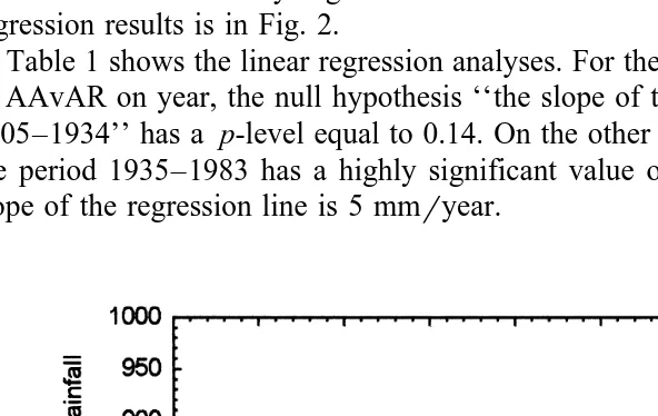
Table 1 shows the linear regression analyses. For the analysis of the linear regression of AAvAR on year, the null hypothesis ‘‘the slope of the regression line is zero during 1905–1934’’ has a p-level equal to 0.14. On the other hand, the p-level of the trend in the period 1935–1983 has a highly significant value of 0.008. During this period, the slope of the regression line is 5 mmryear.
Table 1
Results of regression analyses between annual rainfall and year
Null hypothesis ‘‘Mean annual rainfall is not related to year’’ is rejected if p-level is-0.01.
Rain gauges Slope p-level r Mean Standard Number
Žmm. error of data
Cordoba Observatory 1873–1934´ 0.50 0.62 0.06 705.0 144.6 62
Cordoba Observatory 1935–1987´ 5.0 0.0005 0.46 743.6 168.5 53
Ž .
AAvAR 1905–1934 4.5 0.14 0.29 707.8 133.9 30
Ž .
AAvAR 1935–1983 5.0 0.0008 0.46 756.1 156.3 49
Ž .
Therefore, during the period with amplifying interdecadal fluctuations 1935–1983 , there is a statistically significant trend in annual rainfall with value 5.0 mmryear. In the period 1905–1934, there was not a statistically significant trend in annual rainfall.
The estimated trend of 4.5 mmryear given by the sample regression for period 1905–1934 is adversely influenced by the length of the time series, which is equal to 30 years. Length of time series has to be larger than twice the length of the 22-year timescale fluctuation to obtain accurate results. Calculation of the trend before 1935 based on data from Cordoba Observatory provides results that are more accurate. The
´
data set from Cordoba Observatory starts at 1873. The time series of annual rainfall in
´
Ž Cordoba Observatory confirms this absence of trend. A linear regression analysis see
´
. Ž
Table 1 between annual rainfall amounts in Cordoba Observatory and year period
´
.
1873–1934 shows that annual rainfall trend, equal to 0.5 mmryear, is not significant during this period at the 1% level. Fig. 3 shows the results of regression analysis. The null hypothesis, ‘‘The slope of the regression between annual rainfall amounts and year, is zero’’, is not rejected at the 1% level. This result supports the previous conclusion on the absence of trend in AAvAR in the period 1905–1934. During the period 1935–1987, the time series of annual rainfall in Cordoba Observatory shows, as expected, a trend of
´
5 mmryear. This is the same as the trend of the AAvAR.
The conclusion is reached that simultaneous to the period during which amplifying
Ž .
fluctuation occurs starting about mid-1930s , there is a trend in annual rainfall. Before the starting of amplifying fluctuation, there is no statistically significant trend.
3.3. Trend produced by decadal and interdecadal fluctuations
this reason, to study trend in the band of wavelet timescale larger than 10 years, the time series of annual rainfall at Cordoba Observatory is used. This is adequate because the
´
correlation coefficient is 0.88 between data from common period of the time series of AAvAR and the time series of annual rainfall in Cordoba Observatory. Comparison of
´
Ž . Ž
Fig. 7 for decomposition of AAvAR and Fig. 9 for decomposition of annual rainfall in .
Cordoba Observatory shows the strong similitude between contributions at wavelet
´
timescales larger than 10 years.
Table 2 shows the results of regression analyses of contribution from the bands of timescales smaller than and greater than 10 years on year. Results indicate that fluctuations in rainfall perturbation with timescale greater than 10 years produce the observed trend in the mean of annual rainfall during 1935–1983. Their contribution is 4.72 mmryear during same period at a significance level of 0.001. Fluctuations with
Ž
timescale less than 10 years contribute only with a trend of 0.33 mmryear p-level of .
test statistics for null hypothesis is 0.78 . Trend of observed annual rainfall is 5.0 mmryear.
Therefore, in central Argentina, an important positive trend in annual rainfall is produced by fluctuations with timescales larger than 10 years. Atmospheric processes
Ž .
related to ENSO El Nino — Southern Oscillation are not contributing significantly to
˜
the generation of this trend in annual rainfall. Contributions from bands of wavelet timescale smaller than and larger than 10 years have a correlation coefficient equal to 0.07. This is not significant even at the 5% level.
These results indicate that the rainfall trend of multidecadal extent observed in the Province of Cordoba starts in conjunction with the excitation of a fluctuation that shows
´
increasing timescale and amplitude. This fluctuation was excited approximately in 1935 with a timescale of about 10 years. By 1981 the fluctuation almost reached a 20-year timescale. Contributions from the band of fluctuations with timescale larger than 10 years explains almost all the trend.
Table 2
Results of regression analyses of annual rainfall for the band of timescales smaller than and greater than 10 years
AR: Annual rainfall. AAvAR: Areal Average of Annual Rainfall. Null hypothesis: Slope is zero. Alternative hypothesis: slope is not zero.
Variable Period Timescale Slope p-level
AR in Cordoba Observatory´ 1873–1934 )10 years 0.42 0.18
AAvAR 1935–1983 )10 years 4.72 -0.0001
AR in Cordoba Observatory´ 1873–1934 -10 years 0.08 0.93
AAvAR 1935–1983 -10 years 0.32 0.79
Time–timescale analysis using the Morlet wavelet indicates that the fluctuation Ž
excited in 1935 does not have precedent in the previous 60 years, since 1873 figure not .
shown .
4. Seasonal variability
In this section, the seasonal variability of the pattern of non-periodic fluctuations is Ž .
analyzed. The following questions are answered: 1 In what seasons the amplifying Ž .
fluctuation excited in the mid-1930s occur? 2 What was the influence of fluctuations at decadal and interdecadal timescales on the trend of seasonal rainfall depending on the season? To study seasonal variability in non-periodic fluctuations, the year was
subdi-Ž . Ž
vided into four 3-month periods. These periods are 1 August to October late
. Ž . Ž . Ž .
winter–early spring , 2 November to January late spring–early summer , 3 February
Ž . Ž . Ž .
to April late summer–early autumn , and 4 May to July late autumn–early winter . We reference to these periods as ‘‘seasons’’ or ‘‘3-month period’’ or ‘‘quarterly of year’’.
Morlet wavelet decomposition of seasonal rainfall shows that the amplifying fluctua-tion is observed only in 3-month periods November to January and February to April. Besides, statistically significant trend occurred in the period 1935–1983 only in same
Ž .
3-month periods see Table 3 . Thus, amplifying fluctuation detection and the trend of seasonal rainfall are restricted to the period of the year from late spring to early autumn after 1935; subsequent analyses are restricted to this period.
Contribution from bands with timescale -10 years and )10 years during the seasons November to January, and February to April is given in Table 4. The length of time series has to encompass at least two cycles of dominant timescales to carry out meaningful analyses of partial contribution from bands of wavelet timescales. To satisfy this requirement, use is made of the time series of areal average of 3-month rainfall for the period 1935–1983; and the same type of time series from Cordoba Observatory for
´
the period 1873–1934.
Table 3
Regression analysis of areal average of 3-month rainfall on year for indicated period of the year
p-level of test statistics corresponds to the null hypothesis: Slope is zero, and alternative hypothesis: slope is
not zero.
Quarterly Period Slope p-level Amplifying fluctuation
Žmmryear. is observed?
August to October 1905–1934 1.24 0.17
1935–1983 y0.31 0.62 No
November to January 1905–1934 1.82 0.30
1935–1983 3.10 0.00039 Yes
February to April 1905–1934 1.35 0.30
1935–1983 2.57 0.00079 Yes
May to July 1905–1934 0.073 0.94
1935–1983 y0.27 0.40 No
statistical significance. That is, fluctuations with a timescale of less than 10 years do not contribute to trend of seasonal rainfall in the indicated 3-month rainfall. Contributions in the band of fluctuation with timescale greater than 10 years are the only ones building the trend in annual rainfall as from 1935. In months November to January, during the period 1873–1934, there was a small trend of y0.9 mmryear. Although statistically significant, this trend is very small compared with trend produced by contribution after 1935. Fig. 10 shows the contribution to 3-month rainfall perturbation from band of fluctuations with timescale greater than 10 years, for indicated period of the year. Descriptions of contribution to rainfall perturbation in the each quarterly from wavelet periods as function of year are shown in Figs. 11 and 12. These figures depict clearly the same amplifying fluctuations seen in Fig. 5 for the variable AAvAR. In the period
Ž .
November to January Fig. 11 , the fluctuation that started in the mid-1930s has a structure composed of fluctuations in bands centered in 13.5 years and 22 years
Table 4
Ž .
Regression analysis of rainfall perturbation contribution from indicated timescale band on year for indicated quarterly of year. Variable of regression on year as indicated
Ž .
SR: seasonal rainfall 3-month rainfall . AAvSR: areal average of seasonal rainfall.
Ž .
Variable Season Period Slope mmryear p-level
NoÕember to January
SR Cordoba Observatory´ Timescale-10 years 1873–1934 0.02 0.97 SR Cordoba Observatory´ Timescale)10 years 1873–1934 y0.91 -0.001
AAvSR Timescale-10 years 1935–1983 0.14 0.84
AAvSR Timescale)10 years 1935–1983 2.96 -0.0001
February to April
SR Cordoba Observatory´ Timescale-10 years 1873–1934 0.013 0.98 SR Cordoba Observatory´ Timescale)10 years 1873–1934 0.28 0.05
AAvSR Timescale-10 years 1935–1983 0.13 0.84
()
O.A.
Lucero,
N.C.
Rodrıquez
r
Atmospheric
Research
52
1999
177
–
193
´
Fig. 11. Contribution to reconstruction of perturbation of 3-month rainfall during November to January from
Ž .
indicated wavelet timescales. Contour lines in mm are: 0, 2, 4, 6, 8, 10, 12, and their negative counterpart.
Ž . Ž .
Negative positive contributions to perturbation of annual rainfall are enclosed by dashed full contours. Line starting at 1935 and connecting several negative and positive centers is the same as in the analysis for AAvAR.
Ž .
timescale; whereas in February to April Fig. 12 , it is seen as a chirp-like fluctuation. We are not implying the existence of a chirp-type generating process as signals looking as chirp-like could be produced also by other mechanisms.
5. Conclusions
An amplifying fluctuation is detected in the time series of annual rainfall, starting
Ž .
about mid-1930s in the province of Cordoba central Argentina . The timescale of this
´
fluctuation initially had a value approximate to 10 years, and increased rapidly to a value of about 20 years. This fluctuation is structured as a train of centers of negative and positive rainfall perturbation alternating in time. A strong positive trend in annual rainfall amount started simultaneously to excitation of amplifying fluctuation. Analyses of contribution to reconstruction of time series of perturbation of annual rainfall amount from bands of wavelet timescale indicate that trend is produced by fluctuations with timescale larger than 10 years. Before 1935, annual rainfall had a stationary mean. After that year, mean annual rainfall in this region is increasing at a rate of 5 mmryear. During the period 1935–1983, the trend produced by contribution from band of fluctuations with timescale greater than 10 years is 4.6 mmryear. The remaining 0.4 mmryear of trend is produced by fluctuations with timescale smaller than 10 years, and it does not have statistical significance.
The amplifying fluctuation in the bands of fluctuations with timescale 10–17 years and 17–27 years, is clearly detected in the 3-month periods November to January, and February to April. These are also the only two 3-month periods with trend statistically significant.
Regression analysis of seasonal rainfall on year indicates that there is a discontinuity in trend between the periods 1873–1934 and 1935–1983. In periods November to January and February to April, fluctuations with timescale larger than 10 years produce a statistically significant trend after 1935. Fluctuations with timescale smaller than 10 years do not contribute in a significant way to trend in these seasons.
Ž .
During the 60 years before wave excitation period 1873–1934 , wavelet analysis does not show another amplifying fluctuation of such strong intensity. Finding what triggered this gargantuan amplifying fluctuation in annual rainfall is an important question for understanding multidecadal climate variability.
Acknowledgements
Ž
Drs. C. Torrence and G. Compo, at the University of Colorado Program in .
Atmospheric and Oceanic Sciences , provided the software for wavelet decomposition of rainfall time series into a diagram ‘‘time–wavelet period’’. This wavelet software is available at http:rrpaos.colorado.edurresearchrwaveletsr. This research was partially
Ž
financed by a research grant from CONICOR The Research Council of Cordoba,
´
. Ž
Argentina . This research paper is also a contribution of the first author Dr. Omar A. .
Lucero to the International Hydrological Program of UNESCO as member of its
Ž .
Working Group for Project 1.4 Climate Change .
References
Daubechies, I., 1994. Ten lectures on wavelets. SIAM, 1994.
Haston, L., Michelson, J., 1994. Long-term central coastal California precipitation variability and relationships to El Nino. J. Clim. 7, 1373–1387.˜
Hu, Q., Woodruff, C.M., Mudrick, S.E., 1998. Interdecadal variations of annual precipitation in the Central United States. Bull. Am. Meteorol. Soc., 221–229.
Latif, M., Barnett, T.P., 1996. Decadal climate variability over the North Pacific and North America: dynamics and predictability. J. Clim. 9, 2407–2423.
Lucero, O., 1995. Characteristics of a rainfall climate change on an urban watershed: the case of Cordoba city´
ŽArgentina . Proceedings of the Ninth Conference on Applied Climatology. Am. Meteor. Soc., Dallas, TX..
Lucero, O., 1998a. Invariance of the design storm in a region under a strong rainfall climate change in mid-latitudes in Argentina. Atmos. Res. 49r1, 11–20.
Lucero, O., 1998b. Effects of the southern oscillation on the probability for climatic categories of monthly rainfall, in a semi-arid region in the southern mid-latitudes. Atmos. Res. 49, 337–348.
Mak, M., 1995. Orthogonal wavelet analysis: interannual variability in the sea surface temperature. Bull. Am. Meteorol. Soc. 76, 2179–2186.
Mallat, S., 1998. A Wavelet Tour of Signal Processing. Academic Press, New York, 571 pp.
Meyers, S.D., Kelly, B.G., O’Brien, J.J., 1993. An introduction to wavelet analysis in oceanography and meteorology, with application to the dispersion of Yanai waves. Mon. Weather Rev. 121, 2858–2866. Morlet, J., 1982. Wave propagation and sampling theory. Geophysics 47, 222–236.
Ž .
Torrence, C., Compo, G., 1998. A practical guide to wavelet analysis. Bull. Am. Meteorol. Soc. 79 1 , 61–78. Trenberth, K.E., Hurrel, J.W., 1994. Decadal atmosphere–ocean variations in the Pacific. Clim. Dyn. 9,
303–319.
Weng, H., Lau, K.M., 1994. Wavelets, period doubling, and time–frequency localization with application to organization of convection over the tropical Western Pacific. J. Atmos. Sci. 51, 2523–2541.