1
TUGAS AKHIR
–
MO 091336
PERANCANGAN PELAT BERPENEGAR TAHAN LEDAKAN
RADITYA DANU RIYANTO
NRP. 4310 100 097
Dosen Pembimbing :
Ir. Handayanu, M.Sc., Ph.D
Yoyok Setyo Hadiwidodo, S.T., M.T., Ph.D
JURUSAN TEKNIK KELAUTAN
Fakultas Teknologi Kelautan
Institut Teknologi Sepuluh Nopember
1
FINAL PROJECT
–
MO 091336
DESIGN OF BLAST RESISTANT STIFFENED PLATE
RADITYA DANU RIYANTO
NRP. 4310 100 097
Supervisors :
Ir. Handayanu, M.Sc., Ph.D
Yoyok Setyo Hadiwidodo, S.T., M.T., Ph.D
DEPARTMENT OF OCEAN ENGINEERING
Faculty of Marine Technology
Institut Teknologi Sepuluh Nopember
DESIGN OF BLAST RESISTANT STIFFENED PLATE
FINAL PROJECT
Submitted in Partial Fulfillment of the Requirement For the Bachelor Degree of Engineering
At
Ocean Engineering Department Faculty of Marine Technology Institut Teknologi Sepuluh Nopember
By:
RADITYA DANU RIYANTO NRP. 4310 100 097
1.
PERANCANGAN PELAT BERPENEGAR TAHAN
LEDAKAN
Nama : Raditya Danu Riyanto NRP : 4310 100 097
Dosen Pembimbing : Ir. Handayanu, MSc, PhD
Yoyok Setyo Hadiwidodo, ST, MT, PhD
Perancangan bangunan lepas pantai haruslah memenuhi beberapa kriteria kondisi termasuk kondisi kecelakaan. Ledakan adalah salah satu kecelakaan yang sangat berbahaya untuk operasional bangunan lepas pantai. Tugas akhir ini akan membahas bagaimana cara merancang pelat berpenegar tahan ledakan yang diaplikasikan di bagian-bagian yang potensial terjadi ledakan berdasarkan DNV RP C204 – Design against accidental loads. Tujuan tugas akhir ini adalah menginvestigasi respon struktur pelat (deformation φ and stress σ) yang terkena beban ledakan; menginvestigasi pengaruh variasi konfigurasi penegar, geometri penegar, dan durasi ledakan terhadap respon struktur pelat; serta merancang pelat berpenegar tahan ledakan. Prosedur pelaksanaannya yaitu pemodelan geometri pelat, validasi meshing menggunakan mesh sensitivity dan perhitungan manual, analisa ledakan dan seluruh analisa menggunakan software ANSYS 14.5. Hasilnya yaitu respon maksimal adalah pelat dengan konfigurasi X dan geometri strip dengan midpoint displacement 75.78 mm dan von misesstress 347.77 MPa, sedangkan respons minimal terjadi pada pelat dengan konfigurasi sejajar dan geometri strip dengan midpoint deformation 59.10 dan stress 347.12 MPa. Dan pelat berpenegar tahan ledakan yaitu pelat dengan konfigurasi sejajar dan geometri T yang mampu mereduksi 36.87% deformasi pelat tanpa penegar dengan berat yang lebih ringan dari konfigurasi yang lain. Berdasarkan kriteria perancangan, redesign tidak perlu dilakukan.
PREFACE
Assalamu’alaikum Wr. Wb.
Alhamdulillah, praise God Allah SWT for all the mercy and for the entire miracle, the author finally finishes his Final Project successfully. This Final Project, entitled “Design of Blast Resistant Stiffened Plate” is a real hard work from college student and will be the pride for the author to present it for the society. Shalawat and Salam always praised to Prophet Muhammad SAW.
Author wants to say thanks for all the help and guidance from all the person mentioned so that the project is finished and the book is on the hand of the readers:
1. My Parents, Dwi Hendrarini and Suyanto Abdul Rachman for the non-stop loving and caring
2. Ir. Handayanu, MSc, PhD as 1st Supervisor
3. Yoyok Setyo Hadiwidodo ST, MT, PhD as 2nd Supervisor
4. Cak No (Mujiono), as Technician of Laboratory of Offshore Structural Dynamic FTK ITS Surabaya
5. All the lecturer at Faculty of Marine Technology, ITS Surabaya
6. Mochammad Ramzi, Novanand Sena Putra, Wahyu Putra, Supriyo Jawoto, as partners at Laboratory of Structural Dynamic FTK ITS Surabaya
7. Indria Oktaviani, for the tireless support 8. All the friends from 2010 batch
9. All my friends, family, and colleagues for the support
As a human, author will never be a perfect writer and so is this book, which is far from perfect. Critics and suggestions are welcome.
Surabaya, August 2014
TABLE OF CONTENTS
LITERATURE REVIEW & BASIC THEORY
2.1 Literature Study 5
2.2 General Behaviors of Plate Bending 6
2.3 Blast Phenomena and Loading 11
2.4 Interaction between Blast and Structure 14
2.5 Properties of Various Explosive Gases 16
2.6 Response of Blast Loaded Structures 17
2.7 Stiffened Plate Design Criteria based on DNV OS-C101 (LRFD Method) 20 2.8 Resistance Curves (Stress-Strain Curve) based on DNV RP C204 22
2.9 Material Behavior under High Dynamic Loading 24
2.10 Solution Methods for Structural Dynamic Analysis 26
2.11 Performance of a Structure against Blast Load 28
2.12 ANSYS Explicit Dynamic Software Modules 30
PROCEDURES & METHODOLOGY
3.1 General Procedures 32
3.2 General Methodology 33
3.3 Meshing Validation Procedures 34
3.4 Meshing Validation Methodology 36
3.5 Plate Sizing Validation Procedures 37
3.6 Plate Sizing Validation Methodology 38
3.8 Blast Analysis Methodology 41
3.9 Design Procedures 42
3.10 Design Methodology 43
RESULT AND DISCUSSION
4.1 Modelling 44
4.2 Analysis Result 55
4.2.1 Modal Analysis 55
4.2.2 General Midpoint Deformation Result 56
4.2.3 General Midpoint Von Mises Stress Value 58
4.3 Discussion 61
4.3.1 Geometry and Material Condition 62
4.3.2 Effect of Stiffener Geometry 66
4.3.3 Effect of Stiffener Configuration 69
4.3.4 Effect of Blast Duration 72
4.3.5 Effect of Mass 73
4.4 Design of Blast Resistant Stiffened Plate 74
4.4.1 Choosing the Best Response Stiffened Plate 74
4.4.2 Calculating Response Parameter 74
4.4.3 Response Criteria Comparison 75
CONCLUSION AND SUGGESTION
5.1 Conclusion 76
5.2 Suggestion 77
LIST OF FIGURES
Figure 1.1 The Accident of Piper Alpha Explosion (BBC.uk, 2010) ... 1
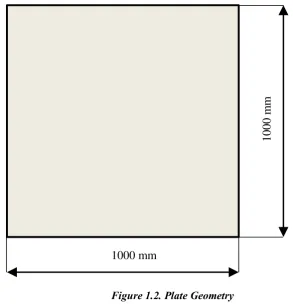
Figure 1.2 Plate Geometry ... 2
Figure 2.1 Plate Deformation General Assumption (Ugural, 1981) ... 6
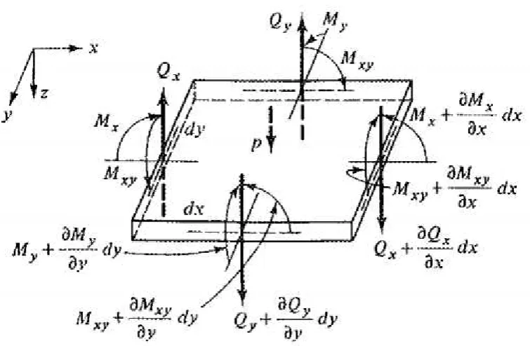
Figure 2.2 Forces and Moments acting on Plate (Ugural, 1981) ... 7
Figure 2.3 Plate Stripping (Ugural, 1981) ... 10
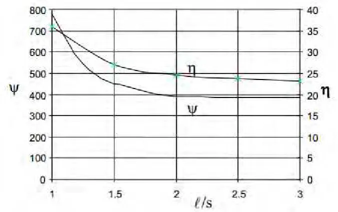
Figure 2.4 Coefficient ψ and η ... 11
Figure 2.5 Blast Wave Propagation (Dusenberry, 2010) ... 12
Figure 2.6 The Typical Load Diagram for (a) Detonation or Shock Wave and (b) Deflagration or Pressure Wave (Dusenberry, 2010) ... 12
Figure 2.7 Simplified (a) Detonation and (b) Deflagration (Merx, 1992) ... 13
Figure 2.8 A schematic representation of the pressure variation (Dusenberry, 2010) ... 16
Figure 2.9 SDOF Analysis Procedure (Su, 2012) ... 19
Figure 2.10 Hexahedron elements with 8 nodes (ANSYS, 2012) ... 20
Figure 2.11 Classification of Resistance Properties ... 23
Figure 2.12 Resistance Curve for ASTM A36 (Bauchio, 1994) ... 23
Figure 2.13 Yield Stress Circle (ANSYS, 2012) ... 25
Figure 2.14 Maximum Plastic Strain Failure (ANSYS, 2012)... 25
Figure 2.15 The Finite Difference Method (Logan, 2007) ... 27
Figure 2.17 Support Rotation ... 30
Figure 2.18 Project Schematics in ANSYS Workbench ... 31
Figure 3.1 Plate Dimension (Tavakoli, 2012) ... 35
Figure 3.2 Boundary Condition ... 35
Figure 3.3 Fixed Ends Boundary Condition Modal Analysis ... 39
Figure 3.4 Analysis setting configuration ... 40
Figure 3.5 Uniform Blast Pressure Load ... 40
Figure 4.1 Meshing Sensitivity Graph ... 51
Figure 4.2 Factored Resistance Curve ... 52
Figure 4.3 Load Profile ... 53
Figure 4.5 Midpoint Deformation 100 ms Blast Duration ... 57
Figure 4.6 Midpoint Deformation 200 ms Blast Duration ... 57
Figure 4.7 Midpoint Von Mises Stress 50 ms Blast Duration... 59
Figure 4.8 Midpoint Von Mises Stress 100 ms Blast Duration... 59
Figure 4.9 Midpoint Von Mises Stress 200 ms Blast Duration... 60
Figure 4.10 Effect of Stiffener Geometry 50 ms ... 67
Figure 4.11 Effect of Stiffener Geometry 100 ms ... 67
Figure 4.12 Effect of Stiffener Geometry 200 ms ... 68
Figure 4.13 Effect of Stiffener Configuration 50 ms ... 69
Figure 4.14 Effect of Stiffener Configuration 100 ms ... 70
Figure 4.15 Effect of Stiffener Configuration 200 ms ... 70
Figure 4.16 Effect Blast Duration ... 72
LIST OF TABLES
Table 2.1 Beam with Various Boundary Condition under Uniform Load P
(Ugural, 1981) ... 9
Table 2.1. Drag Coefficient on Various Shapes (Dusenberry, 2010 ... 15
Table 2.2. Properties of Explosive Gases (Hall, 1985) ... 16
Table 2.3. Load and Resistance Factor for ALS... 22
Table 2.5. Level of Protection Criteria ... 28
Table 2.6. Component Damage Levels ... 29
Table 2.7. Response Criteria (Dussenberry, 2010) ... 30
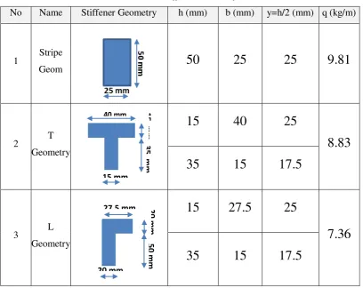
Table 3.1. Stiffener Geometr ... 37
Table 3.2. Selected Structure Protection Level ... 42
Table 3.3. Selected Structure Damage Level ... 42
Table 3.4. Selected Response Parameter... 43
Table 4.1. Stiffener Geometry and Section Modulus ... 45
Table 4.2. Geometry Modelling ... 46
Table 4.3. Model Validation and Meshing Sensitivity ... 50
Table 4.4. Weight Calculation and Ratio ... 51
Table 4.5. Material Properties ... 52
Table 4.6. Resistance Curve Table ... 52
Table 4.7. Propane Gas Explosion Properties ... 53
Table 4.8. Analysis Matrix ... 54
Table 4.9. Natural Period and Analysis Region ... 55
Table 4.10. Maximum Midpoint Deformation Value ... 58
Table 4.11. Maximum Midpoint Deformation Value ... 61
Table 4.12. Geometry and Material Condition, Unstiffened Plate 50 ms ... 63
Table 4.13. Geometry and Material Condition, Geometry Stripe 100 ms ... 64
Table 4.14. Geometry and Material Condition, Config T Geom T, 100 ms ... 65
Table 4.15. Geometry and Material Condition, Config L Geom Par,200 ms ... 66
Table 4.16 Stiffener Geometry Reduction at 50 ms Blast Duration ... 68
Table 4.17 Stiffener Geometry Reduction at 100 ms Blast Duration ... 68
Table 4.19 Summary of Stiffener Geometry Reduction ... 69
Table 4.20 Stiffener Configuration Reduction at 50 ms Blast Duration ... 71
Table 4.21 Stiffener Configuration Reduction at 100 ms Blast Duration ... 71
Table 4.22 Stiffener Configuration Reduction at 200 ms Blast Duration ... 71
Table 4.23 Summary of Stiffener Configuration Reduction ... 71
Table 4.24 Effect of mass variation ... 73
Table 4.25 Best response stiffened plate ... 74
Table 4.26 Response Parameter Calculation ... 74
LIST OF NOTATIONS
φ deformation (mm)
σ stress (MPa)
ρ density (kg/m3)
t plate thickness (mm)
Lx plate width in x direction (mm) Ly plate width in y direction (mm) D plate bending stiffness (kg.mm2) P(t) Overpressure at time t (kg/mm2) Ps Maximum Overpressure (kg/mm2) mü Inertial coefficient
bu̇ Damping coefficient ku Restoring coefficient
f(t) Excitation Force (kg/mm2) I Moment of Inertia (Area) (mm4)
S Section Modulus (mm3)
F Frequency (Hz)
1
SECTION I
INTRODUCTION
1.1
Background
The design of offshore structure should satisfy several conditions including the extreme loading condition. Extreme loading condition, also known as Accidental Load, consist of Dropped Object, Ship Collision, Fire Hazard, and Blast Hazard (DNV, 2012). Dropped object is the accident when the shackle or sling of lifted object is broken causing object move freely downward and hit the topside structure. Ship collision is when the platform hit by ship and causing the severe damage to the structure. Fire and blast hazard are mainly caused by the leakage of processing/power component.
The blast hazard is the one most dangerous accident that could happen on the offshore structure operation. Blast is a pressure disturbance caused by the sudden release of energy. People often think of blasts in terms such as the detonation of an explosive charge. However, there are many other blast sources that have the potential to cause damage. For example, chemicals may undergo a rapid decomposition under certain conditions. Flammable materials mixed with air can form vapor clouds that
2
when ignited can cause very large blasts. Blasts are not always caused by combustion; they can also result from any rapid release of energy that creates a blast wave, such as a bursting pressure vessel from which compressed air expands, or a rapid phase transition of a liquid to a gas (Dusenberry, 2010). There are many case of blast accident that leads a facility to total damage and loss of life, both land-based structures like Fukushima Nuclear Reactor accident or offshore structure like Piper Alpha accident. The accident of Piper Alpha, 1988, an offshore platform at North Sea, collapsed after a series of gas blast. The Piper Alpha Platform was designed without considering the blast load, killing 169 men and total capital loss of US$ 1.7 million (McGinty, 2010). These accidents are strong evidence that a blast resistant structure is important so that would be no casualties regarding to this type of accident in the future.
This project will provide a method to build a panel of stiffened plate that resists to a blast loading based on DNV RP C204 – Design against accidental loads; it can be applied to cover vulnerable area that has a potential blast accident. As stated by Rajendran and Lee (2008), stiffened plate structure is widely used at marine industry such as ship hull or offshore topside structure. This project will vary the stiffener configuration and blast duration to gain the best stiffener configuration and the effect of blast duration to the structure. This may lead us to a safer design of offshore structures, especially the stiffened plate structures.
1.2
Problems
This project will focus on solving the problems:
1. How are the midpoint responses (deformation φ and stress σ) of varied stiffened plate subjected to blast loading?
2. How are the variation of stiffener geometry, stiffener configuration, and blast duration affect the responses?
3
1.3
Purpose
This project aims to:
1. Calculate the midpoint responses (deformation φ and stress σ) of plate subjected to blast loading.
2. Investigate the effect of stiffener geometry, stiffener configuration, and blast duration to the responses.
3. Design a blast resistant stiffened plate based on the best stiffener configuration response result.
1.4
Benefit
The motivation for this project arises from primary concern for the design of plate structures against blast loads. Through this project, hopefully there will be a better understanding of blast load characteristic and creates a safer design of stiffened plate against blast load.
1.5
Limitation
This project, in order to focus on the design calculation and for the sake of simplicity, limited by these condition:
1. The material properties of plates are based on ASTM A36 with yield stress at 36 ksi (255 MPa).
4
Figure 1.2. Plate Geometry
3. The stiffeners properties are 25 mm thick and 50 mm height as the preliminary design size and limited into 2 pieces, the shape will be varied on
“T”, “L” and stripe configuration.
4. The finite element analysis tool used is ANSYS Explicit Dynamic Modules. Each edge of the plate considered as fixed support.
5. The blast loading modeled as simplified time history dynamic pressure. The
pressure are fixed at vapor density ρ=1.240 kg/m3 , that is the vapor density of propane gas explosion (Hall, 1985) and varied at time 50, 100, and 200 ms. 6. The Recommended Practice to be used is DNV RP C204-Design against
Accidental Loads.
7. The Design Criteria to be used is DNV OS C101-Design of Offshore Steel Structure, General (LRFD Method)
8. The structural steel resistance curve is an elastic-perfectly plastic curve with strain hardening.
9. The overlapping and weldability of the stiffener configuration crossing is neglected (Kadid, 2008).
10.The critical damping ratio is set at 0.10 1000 mm
1000
m
5
2.
SECTION II
LITERATURE REVIEW & BASIC THEORY
2.1
Literature Study
There has been an increased activity in blast loading research in the last two decades. Most of these were empirical research, but in recent years, modern computers and powerful finite element packages, facilitate the numerical study.
Comparison between experimental and numerical responses of steel plates subjected to air blast loads has been indicated the accuracy of modern calculation methods and computational codes. Modern computational codes can predict the dynamic response of unstiffened plates accurately, specially the forced vibration phase and the first pulses of the response. However, there are differences between different codes because its shell elements definition. These differences could result in different predictions, particularly in free vibration phase and in nonlinear studies (Jacinto, et al., 2001).
A numerical investigation generated by Kadid (2008) and Tavakoli (2013), by modelling some varied stiffened plates subjected to uniform blast loading. In this paper the nonlinear dynamic response of square steel stiffened plates subjected to uniform blast loading was studied. Stiffener configurations and boundary conditions, which maybe affect the dynamic response of the plates subjected to blast loading was considered.
6
2.2
General Behaviors of Plate Bending
Plates and shells are initially flat and curved structural elements, respectively, for which the thicknesses are much smaller than the other dimensions.
t << Lx, Ly (1)
Included among the more familiar examples of plates are table tops, street manhole covers, side panels and roofs of buildings, turbine disks, bulkheads and tank bottoms. Many practical engineering problems fall into categories “plates in bending" or “shells in bending." Plates may be classified into three groups: (a) thin plates with small deformations, (b) thin plates with large deformations, and (c) thick plates. According to the criterion often applied to define a thin plate (for purposes of technical calculations) the ratio of the thickness to the smaller span length should be less than 1/20 (Ugural, 1981)
Figure 2.1. Plate Deformation General Assumptions (Ugural, 1981)
7 a) The deformation of the midsurface is small compared with the thickness of the plate. The slope of the deflected surface is therefore very small and the square of the slope is a negligible quantity in comparison with unity.
b) The midplane remains unstrained subsequent to bending.
c) Plane sections initially normal to the midsurface remain plane and normal to that surface after the bending. This means that the vertical shear strains γxz and γyz, are negligible.
d) The stress normal to the midplane is small compared with the other stress components and may be neglected.
2.2.1
Governing Equation of Plate Deformation
The components of stress generally vary from point to point in a loaded plate. These variations are governed by the conditions of equilibrium of statics. Fulfillment of these conditions establishes certain relationships known as the equations of equilibrium.
Figure 2.2. Forces and Moments acting on Plate (Ugural, 1981)
8
over each face, in the figure they are shown by a single vector, representing the mean values applied at the center of each face. With change of location, as for example, from upper left corner to the lower right corner, one of the moment components, say Mx acting on the negative x face, varies in value relative to the positive x face. This variation with position may be expressed by a truncated Taylor's expansion in
From the state above we can build the plate deformation governing equation:
The equation above is firstly stated by Lagrange in 1811 (Ugural, 1981), can also be written in concise form:
𝛻4𝑤 = 𝑝
9
2.2.2
Strip Method to Solve Rectangular Plate with Arbitrary
Boundary Condition under Various Loading
H. Grashof stated an efficient way for computing deformation and moment in a rectangular plate with arbitrary boundary conditions (Ugural, 1981). This so-called strip method that is the plate is assumed to be divided into systems of strips, each strip regarded as functioned as a beam. The method permits qualitative analysis of the plate behavior with ease but is less adequate, in general, in obtaining accurate quantitative results.
Note, however, that because this method always gives conservative values for both deformation and moment, it is often employed in practice. A very efficient engineering approach to design of the rectangular floor slabs is also based upon the strip method. Before proceeding to a description of the method, it will prove useful to introduce maximum deformation and moments of a beam with various end conditions. Expressions for such quantities for a beam of length L subjected to a uniform load p, derived from the mechanics of materials, are given in table below:
Table 2.1. Beam with Various Boundary Condition under Uniform Load P (Ugural, 1981)
10
Figure 2.3. Plate Stripping (Ugural, 1981)
System (a) is the stripped plate and each fraction threatened as beam and (b) is the original state condition. Note that these following conditions should be applied to obtain the bending moments and the deformation:
Wa = wb and P0 = Pa + Pb at (x = y = 0)
DNV RP-C204 gives more accurate calculations rigid plastic theory combined with elastic theory that may be used. In the elastic range the stiffness and fundamental period of vibration of a fixed plate under uniform lateral pressure can be expressed as:
11
Figure 2.4. Coefficient ψ and η
2.3
Blast Phenomena and Loading
12
Figure2.5. Blast Wave Propagation (Dusenberry, 2010)
Blasts are separated into two types; (a) detonations and (b) deflagrations. A typical gas explosion is of the deflagration type, while an explosion of condensed explosives (or a very powerful gas explosion) is in the detonation range.
Figure2.6. The Typical Load Diagram for (a) Detonation or Shock Wave and (b) Deflagration or Pressure Wave (Dusenberry, 2010)
13 The detonation empirical function as provided by Bangash (2012) is widely accepted, this equation also used by Spranghers (2012) and Vantomme (2012) for measuring aluminum plates under blast load:
𝑃(𝑡) = 𝑃0+ 𝑃𝑠(1 −𝑡𝑇𝑝) 𝑒(−
𝑎𝑡
𝑡𝑝) (7)
Where:
P(t) = Overpressure at time t (kg/m2) Ps = Maximum Overpressure (kg/m2)
t = Time (s)
tp = Blast duration (s)
a = Negative time constant
The maximum value of this negative pressure does not normally play any important role, since this pressure is of a magnitude much smaller than the positive peak overpressure. A deflagration is characterized by a rise time, and a slower decrease to zero within the positive phase duration time. A common simplification of the shape of the pressure diagrams is to linearize the variation, as shown in figure below, as provided by Merx (1992):
Figure 2.7. Simplified (a) Detonation and (b) Deflagration (Merx, 1992)
14
because the maximum overpressure and blast positive duration has the same value as the empirical ones. The simplified blast load (triangular load) is stated as follow:
𝑃(𝑡) = 𝑃𝑠(1 −𝑡𝑡 deflagration is stated as follow:
𝑃(𝑡) = {𝑃𝑠 (
2.4
Interaction between Blast and Structure
A blast, when meeting a structure or an obstacle creates a dynamic load on the structure. This is caused by air displacement in the direction of the blast-wave. The air displacement from a blast is referred to as an explosion wind, and causes a dynamic overpressure given by the following formula:
𝑃𝑠 = 12× 𝐶𝐷× 𝜌𝑠× 𝑣𝑠2 (10)
Where:
Ps = Dynamic Overpressure (Pa) CD = Drag Coefficient
15
𝑣𝑠 = Blast wave propagating velocity (m/s)
CD is drag coefficient which is dependent on the shape of the structure (projected area) and its orientation relative to the blast front.
Table 2.2. Drag Coefficient on Various Shapes (Dusenberry, 2010)
16
represents a case where the blast wave runs over a large surface without hindrance. The load on the surface will for this case be taken equal to the overpressure PS of the incident wave. In case (B), the blast wave is on a path perpendicular to a surface of very large dimensions. There will be minimal rarefaction effects from the edges, and the load on the surface can be taken as the overpressure from the reflected blast wave Pr. For case (C) we are dealing with an object of small dimensions, the rarefaction progresses so quickly that any reflection can be neglected. Furthermore, one can assume that the pressure difference between the front and back part of the part is so small that only the dynamic pressure PD is considered. It should be noted that in most structures, a combination of these three cases must be considered.
Figure 2.8. A schematic representation of the pressure variation (Dusenberry, 2010)
2.5
Properties of Various Explosive Gases
The blast wave is mainly influenced by gas density and deflagration velocity. Hall et. al. (1985) studied the behavior of hydrocarbon explosion in free air.
Table 2.3. Properties of Explosive Gases (Hall, 1985)
Gas Density (kg/m3) Energy Release per Unit Volume (MJ/m3)
Blast Velocity (m/s)
Acetylene C2H2 1.223 1.503 1,830
Ethylene C2H4 1.225 1.348 1,705
Propane C3H8 1.240 1.238 1,660
Methane CH4 1.198 1.204 1,590
Ammonia NH3 1.151 1.063 1,095
17 The typical vapor gas blast duration at petrochemical facilities is at 50 up to 200 ms (Su, 2012). The effect of duration variation is the most important to be accounted for, due to the short-and-heavy load characteristic of blast load, and it is implies the magnitude of impulse generated from the loads.
2.6
Response of Blast Loaded Structures
The response of structural components can conveniently be classified into three categories according to the duration of the explosion pressure pulse, td, relative to the natural period of vibration of the component, T (DNV, 2012):
Impulsive domain td/T < 0.3 Dynamic domain 0.3 < td/T < 3 Quasi-static domain td/T > 3 Impulsive domain:
The response is governed by the impulse defined by:
𝐼 = ∫ 𝐹(𝑡)𝑑𝑡𝑡𝑑
0 (11)
Hence, the structure may resist a very high peak pressure provided that the duration is sufficiently small. The maximum deformation, wmax, of the component can be calculated iteratively from the equation:
𝐼 = √2𝑚𝑒𝑞∫0𝑤𝑚𝑎𝑥𝑅(𝑤)𝑑𝑤 (12)
Where:
R(w) = Force-deformation relationship for the component meq = Equivalent mass for the component
Quasi-static domain:
The response is governed by the peak pressure and the rise time of the pressure relative to the fundamental period of vibration. If the rise time is small the maximum deformation of the component can be solved iteratively from the equation:
18
If the rise time is large, the maximum deformation can be solved from the static condition:
𝐹𝑚𝑎𝑥 = 𝑅(𝑤𝑚𝑎𝑥) (14)
Dynamic analysis:
The response has to be solved from numerical integration of the dynamic equation of equilibrium. In most cases, the domain of blast duration is at dynamic region.
2.6.1
Dynamic Analysis of Blast Loaded Structure
Dynamic analysis is characterized by the time variant change of both loading and response. The solution of dynamic response should account for all time variant response and form it as a time history result. In general, dynamic equilibrium equation is stated as follow:
𝑚𝑢̈(𝑡) + 𝑏𝑢̇(𝑡) + 𝑘𝑢(𝑡) = 𝑓(𝑡) (15)
Where:
𝑚𝑢̈(𝑡) = Inertial force, the product of mass and acceleration
bu̇(t) = Damping force, the product of viscous damping
𝑘𝑢(𝑡) = Restoring force, the product of stiffness constant K and displacement
𝑓(𝑡) = Excitation Force
An object subjected to the blast loading could be modelled as SDOF or MDOF system (DNV, 2012).
a. SDOF System – Continuous System
19
𝑘 = ∫ 𝐸𝐼(𝜑′′)𝑙 2𝑑𝑥
0 + ∫ 𝑘(𝑥𝜑2)𝑑𝑥 + ∑ 𝐾𝑛𝑖 𝑖𝜑𝑖 𝑙
0 = generalized stiffness (18)
𝑝(𝑡) = ∫ 𝑞(𝑥, 𝑡)𝜑𝑑𝑥 + ∑ 𝐹0𝑙 𝑛𝑖 𝑖𝜑𝑖 = generalized excitation force (19)
Where φ is the assumed shape function, the integral parts show the continuous form of the system while the Σ shows the several discrete elements or forces may be present.
Figure 2.9. SDOF Analysis Procedure (Su, 2012)
b. MDOF System
For scenarios such as a topside frame structure being exposed to a blast load, the problem can no longer be simplified as a SDOF-system, and more advanced methods have to be implemented. The most common method is to use the Finite Element Method (FEM)/Finite Element Analysis (FEA), utilizing its ability to handle complicated geometries and boundaries. The Finite Element Analysis (FEA) will divide the system into elements based on mesh setting on the solver software. Meshing is the process to divide the plates and stiffeners into small elements and solve the numerical integration. This process will integrate these following equations:
{𝐹(𝑡)} = [𝐾]{𝑑} + [𝐵]{𝑑̇} + [𝑀]{𝑑̈} (20)
Where:
[𝐾] = ∑ [𝑘𝑁𝑖=1 𝑖] = Stiffness Matrix
20
[𝑀] = ∑ [𝑚𝑁𝑖=1 𝑖] = Inertial Matrix
{𝐹} = ∑ {𝑓𝑁𝑖=1 𝑖} = Excitation Force Matrix
The matrices consist of hexahedron elements with 8 nodes (ANSYS, 2010):
Figure 2.10. Hexahedron elements with 8 nodes (ANSYS, 2012)
2.7
Stiffened Plate Design Criteria based on DNV OS-C101-Design of
Offshore Steel Structure, General (LRFD Method)
Design criteria chosen on this project is DNV OS-C101-Design of Offshore Steel Structure, LRFD method. LRFD method provides fairer loading by multiplying both loads and resistance to create safer design and yet give economically beneficial result. (bgstructuralengineering.com, 2008)
2.7.1
Design criteria for plates and girders
a. General Design Format using LRFD Method
The level of safety of a structural element is considered to be satisfactory if the design load (Sd) does not exceed the design resistance (Rd).
Sd ≤ Rd (21)
Or:
21 Where the design load factor
γ
f and design resistance factorφ
is determined by specific limit state condition, in this case, the limit state used is ALS (Accidental Limit State).b. Minimum Dimension for Plate and Girders
The thickness of plate subjected to lateral pressure shall not be less than:
𝑡 = 14.3𝑡0
√𝑓𝑦𝑑 (𝑚𝑚) (23)
Where:
𝑓𝑦𝑑 = design yield strength (N/mm2),
= fy/γm
𝑡0 = 7 mm for primary structural elements
γm = material factor = 1.15 for steel
The section modulus Ss for longitudinals, beams, frames and other stiffeners subjected to lateral pressure shall not be less than:
𝑆𝑆 = 𝑙
2𝑠𝑝𝑑
𝑘𝑚𝜎𝑝𝑑𝑘𝑝𝑠 10
6(𝑚𝑚3), 𝑚𝑖𝑛𝑖𝑚𝑢𝑚 15.103(𝑚𝑚3) (24)
l = stiffener span (m) km = bending moment factor
= 12 for fixed ends
σpd = design bending stress (N/mm2) kps = fixity parameter for stiffeners
= 1.0 if at least one end is fixed
2.7.2
Accidental Limit States (ALS)
As stated by DNV (2011), structures shall be checked in ALS in two steps: a) Resistance of the structure against design accidental loads
22
caused by the design accidental loads (the response exceeds elastic region of the material).
DNV also states that if non-linear, dynamic finite element analysis is applied for design, it shall be verified that all local failure mode, e.g. strain rate, local buckling, joint overloading, joint fracture, are accounted for explicit evaluation.
a. Load and Resistance Factor for ALS
For Accidental Limit State, the load and resistance factors are defined below: Table 2.4. Load and Resistance Factor for ALS
No. Parameter Value Remarks
1.
γ
f 1.0 Load factor2. Fk Calculated Characteristic loads
3.
φ
1𝛾𝑚 Resistance factor
4. 𝛾𝑚 1.15 Material factor for steel
5. Rk Based on resistance curve
for each material Characteristic resistance
2.8
Resistance Curves (Stress-Strain Curve) based on DNV RP
C204-Design against Accidental Loads
23
Figure 2.11. Classification of Resistance Properties
Elastic: Elastic material, small deformations.
Elastic-perfectly plastic: Elastic perfectly plastic material. The material characteristic after the strain exceeds the elastic region remains plastic (k2). Elastic-plastic with strain hardening: Elastic-perfectly plastic material. The
material characteristic after the strain exceeds the elastic region remains plastic (k2) until reaching the strain hardening region (k3).
DNV (2010) states that in designing the structures to resist the accidental loads, the effect for strain hardening has to be accounted. And the value of each response should be multiplied by resistance factor as stated in point 2.7.2.a. This figure below represent the resistance curve for ASTM A36 steel, with strain hardening considered, as provided by Bauchio (1994):
Figure 2.12. Resistance Curve for ASTM A36 (Bauchio, 1994)
24
2.9
Material Behavior under High Dynamic Loading
In general, materials have a complex response to dynamic loading. The following phenomena needs to be modelled (ANSYS, 2012):
2.9.1
Material Plasticity
If a material is loaded elastically and subsequently unloaded, all the deformation energy is recovered and the material reverts to its initial configuration. If the deformation is too great a material will reach its elastic limit and begin to deform plastically. In Explicit Dynamics, plastic deformation is computed by reference to the Von Mises yield criterion (also known as Prandtl–Reuss yield criterion). This states that the local yield condition is:
(𝜎1− 𝜎2)2+ (𝜎2− 𝜎3)2+(𝜎3− 𝜎1)2 = 2𝑌2 (25)
Where the “Y” is the yield stress in simple tension. It can be also written as:
𝜎
12+ 𝜎2
2+ 𝜎3
2=
2𝑌2
3 because
𝜎
1+ 𝜎
2+ 𝜎
3= 0
In ANSYS, if an incremental change in the stresses exceeds the Von Mises criterion, then each of the principal stress deviators must be adjusted such that the criterion is satisfied. If a new stress state n + 1 is calculated from a state n and found to fall outside the yield surface, it is brought back to the yield surface along a line normal to the yield surface by multiplying each of the stress deviators by the factor C:
𝐶 = (23)1/2𝑌
(𝜎12+𝜎22+𝜎32)1/2 (26)
25
Figure 2.13. Yield Stress Circle (ANSYS, 2012)
During the material modelling in ANSYS, this plasticity behavior is represented by bilinear or multilinear hardening. Bilinear hardening refers to elastic-perfectly plastic resistance curve. The multilinear hardening is the customized stress-strain relationship; user can define up to 10 stress-strain relationship.
2.9.2
Material Failure
When stress occurred in the structure exceeds the strain limit of the material, the failure will happen. After failure initiation, subsequent strength characteristics will change depending on the type of failure model. In ANSYS, there are several failure models representing the material failure:
a. Plastic Strain Failure
26
Figure 2.14. Maximum Plastic Strain Failure (ANSYS, 2012)
b. Principal Stress/Strain Failure
This failure will occur when the maximum tensile stress/strain or shear stress/strain exceeded. The ANSYS standard maximum value is 1x10²⁰.
2.10
Solution Methods for Structural Dynamic Analysis
In FEA (Finite Element Analysis), direct numerical integration methods are used to find approximate solutions to the response problems. These are considered standard solution methods for most FEA Software e.g. ANSYS (Su, 2012). These procedures will enable us to determine the nodal displacements at different time increments for a given dynamic system. The direct numerical integration methods are separated into two methods; implicit and explicit methods. The first is an explicit method known as the central difference method. The second is the implicit methods known as the Newmark-Beta (or Newmark’s) method (Logan, 2007).
2.10.1
Explicit Method (Central Difference Method)
The central difference method is based on finite difference expressions in time for velocity and acceleration at time (t) given by (Logan, 2007):
𝑑̇ =𝑖 𝑑𝑖+12(∆𝑡)−𝑑𝑖−1 … (27)
𝑑𝑖̈ = 𝑑
27
Figure 2.15. The Finite Difference Method (Logan, 2007)
The steps of iteration to get obtain the deformation based on the explicit method are: 1) Given the initial condition 𝑑0̈ , 𝑑0̇ , 𝑑0, and f(t)
2) Solve the deformation for the −∆𝑡
𝑑−1 = 𝑑0− (∆𝑡)𝑑0̇ +(∆𝑡) 2
2 𝑑0̈
3) Solve the deformation for the time t that is ti − ∆𝑡
𝑑𝑖−1 = 𝑀−1{(∆𝑡)2𝐹0+ [2𝑀 − (∆𝑡)2𝐾]}𝑑0− 𝑀𝑑−1
4) Solve the deformation for the time 𝑡𝑖 + ∆𝑡
𝑑𝑖+1 = 𝑀−1{(∆𝑡)2𝐹1+ [2𝑀 − (∆𝑡)2𝐾]}𝑑1− 𝑀𝑑0
5) Solve the acceleration at ti − ∆𝑡 and 𝑡𝑖 + ∆𝑡
𝑑𝑖−1̈ = 𝑀−1(𝐹𝑖−1− 𝐾𝑑𝑖−1)
𝑑𝑖+1̈ = 𝑀−1(𝐹𝑖+1− 𝐾𝑑𝑖+1)
6) Solve the velocity at 𝑡𝑖 + ∆𝑡
𝑑̇𝑖+1 = 𝑑𝑖+12(∆𝑡)−𝑑𝑖−1 (28)
28
2.11
Performance of a Structure against Blast Load
Blast design and analysis are primarily component-based, whereby the applied blast load and response of each component in the building are determined individually. However, performance goals are usually set in terms of life safety, functionality, and reusability for the entire building (Dussenberry, 2010). Therefore, damage or response levels for individual building components must be established to achieve the overall building performance. In this approach, a building Level of Protection is selected based on desired performance goals, as shown in Table 2.4. Table 2.5 is then used to determine the associated damage levels for each type of component in the building. Therefore, this approach determines component damage levels that are consistent with an overall building performance goal. It can also be used to assess the Level of Protection provided by an existing building, based on calculated component damage levels.
Table 2.5. Level of Protection Criteria Level of
Protection
Structure Performance Goals Overall Structure Damages
I(Very low) Collapse prevention: Surviving occupants will likely be able to evacuate, but the building is not reusable; contents may not remain intact. only temporarily; contents will likely remain intact for retrieval.
Damage is expected, such that the building is not likely to be economically repairable, but progressive collapse is unlikely. III (Medium) Property preservation: Surviving
occupants may have to evacuate temporarily, but will likely be able to return after cleanup and repairs to resume operations; contents will likely remain at least partially functional, but may be impaired for a time.
Damage is expected, but building is expected to be economically repairable, and progressive collapse is unlikely.
IV (High) Continuous occupancy: All occupants will likely be able to stay and maintain operations without interruption
29 Table 2.6. Component Damage Levels
Level of
I(Very low) Heavy Hazardous Hazardous
II (Low) Moderate Heavy Heavy
III (Medium) Superficial Moderate Moderate
IV (High) Superficial Superficial Superficial
Hazardous damage—The element is likely to fail and produce debris.
Heavy damage—The element is unlikely to fail, but will have significant permanent deformation such that it is not repairable.
Moderate damage—The element is unlikely to fail, but will probably have some permanent deformation such that it is repairable, although replacement may be preferable for economic or aesthetic reasons.
Superficia damage—The element is unlikely to exhibit any visible permanent damage
2.11.1
Response Parameter and Criteria
The response parameters define the structure damage level. As stated by Dussenberry (2010) the response parameter of structure under blast loading are:
a. Support Rotation (θ)
Support rotation parameter is calculated by:
𝜃 = 𝑡𝑎𝑛−1(2𝑥𝑚
𝐿𝑚𝑖𝑛) (29) Where:
xm = maximum deformation
30
Figure 2.17. Support Rotation
b. Ductility Limit (µ)
Ductility limit is calculated by:
𝜇 =𝑋𝑚
𝑋𝑦 (30) Where: Xm = Maximum Deformation
Xy = Deformation at yield stress
The response criteria limits the value of response parameter so that the structure can be assessed and categorized as a blast resistant structure. Table 2.6 defines the response criteria:
Table 2.7. Response Criteria (Dussenberry, 2010)
Component
2.12
ANSYS Explicit Dynamic Software Modules
31 flows, failure), from contact (for example, high speed collisions and impact) and from the geometric deformation (for example, buckling and collapse). Events with time scales of less than 1 second (usually of order 1 millisecond) are efficiently simulated with this type of analysis (for example, blast analysis) (ANSYS, 2012). ANSYS Explicit Dynamics is one of the Workbench Modules that allows the designer has the step-by-step analysis starting from the model input, setting up the analysis condition, executing the analysis and reviewing the result easily thanks to the project schematics method.
Figure 2.18. Project Schematics in ANSYS Workbench
32
3.
SECTION III
PROCEDURES & METHODOLOGY
3.1
General Procedures
The steps to do to obtain the result of this project will be as follows: 1. Literature study to obtain the data and supporting theory.
2. Modelling the stiffened plate structure using external CAD software and then importing the model to ANSYS Workbench Design Modeler, AutoCAD 2013 is chosen to support the Design Modeler. There will be 9 sets of models to be generated, namely 3 variations of stiffener geometry and 3 variations of stiffener configuration.
3. Obtaining the natural period for each model using ANSYS Workbench Modal Analysis.
4. Validating the model by hand calculation using simplified SDOF analysis and meshing sensitivity of natural period. If the natural period doesn’t exceed 5% deviation, the model considered as a valid plate model. Meshing sensitivity is the iterative steps to obtain the stable result at certain mesh sizing. The weight for each model will be calculated and expected to be equal for the sake of fair comparison. The deviation tolerance is 15%.
5. Calculating t/td. The criteria for analysis setting is: Impulsive domain td/T < 0.3 Dynamic domain 0.3 < td/T < 3 Quasi-static domain td/T > 3
6. Analyzing the model based on the validity region, giving the dynamic blast pressure at various durations and obtaining the result data using ANSYS Workbench Explicit Dynamic Modules.
33
not exceed the design criteria the plate considered as a proper design of stiffened plate that resist to blast load.
8. Conclusion.
3.2
General Methodology
Start
Stiffened Plate Modelling:
Varying the stiffener geometry Varying the stiffener configuration
Modal Analysis to obtain the natural period
Natural Period Validating No
Literature Study: Blast Loading Profile Plate and Stiffener profile Design Criteria
Weight Validating No
Yes
A B
34
3.3
Meshing Validation Procedures
1. Modelling the unstiffened plate with provided geometry and materials, taken from paper by Tavakoli, (2012), the geometry modelled using AutoCAD 2013 then exported to ANSYS Design Modeler and dimension is as follow:
Blast Loading: Varying the blast duration
Code Checking: Deformation Stress
Yes No
Finish
A B
td/T calculation, validity region is as follow: Impulsive domain td/T < 0.3
Dynamic domain 0.3 < td/T < 3 Quasi-static domain td/T > 3
Good Design Choosing the best response
35
Figure 3.1. Plate Dimension (Tavakoli, 2012)
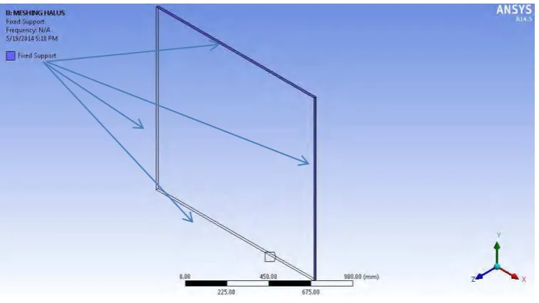
2. Importing the ANSYS Design Modeler file to ANSYS Modal Analysis and then apply the boundary condition, fixed support at the edges of plate:
Figure 3.2. Boundary Condition 1200 mm
1200
m
m
36 3. Running the modal analysis with boundary condition stated at point 2 from
coarse meshing (120 mm size) with decrement of meshing size 20 mm. 4. Analyzing the 1st shape mode natural period per meshing size.
5. Compare the result to the Tavakoli’s model and hand calculation developed by DNV, as stated at equation (6). The deviation tolerance is 5%.
6. Choose the best meshing size based on the comparison.
3.4
Meshing Validation Methodology
Start
Unstiffened Plate Geometry Data
Plate Modelling
Boundary Condition
Modal Analysis
Hand Calculation
Comparing the results. Deviation
tolerance 5%
37
3.5
Plate Sizing Validation Procedures
1. Given initial plate span 1000 mm x 1000 mm.
2. Calculating plate thickness using equation developed by DNV as stated at equation (23).
3. Given initial stiffener dimension, b x h = 25 mm x 50 mm 4. Modifying stiffener geometry into “T” and “L” geometry:
Table 3.1. Stiffener Geometry
5. Calculating minimum stiffener section modulus by equation developed by DNV as stated at equation (24).
6. Calculating the weight of each stiffened plate and then compared to the average weight. The deviation should not be more than 15%.
7. The plate geometries are ready to be analyzed.
38
3.6
Plate Sizing Validation Methodology
Start
Initial Plate and Stiffener Geometry
Calculating plate thickness
Calculating stiffener section modulus
Code check
Plate ready Yes No
Calculating plate weight
39
3.7
Blast Analysis Procedures
1. Modal analysis to obtain 1st mode natural period (T). Modal analysis performed using ANSYS Modal Analysis with fixed ends boundary condition.
Figure 3.3. Fixed Ends Boundary Condition Modal Analysis
2. Importing the model from ANSYS Design Modeler to ANSYS Explicit Dynamic.
3. Determining the material behavior, resistance curve and failure model of the material, as stated at chapter 2.9.
4. Determining blast duration (td) and peak overpressure (Ps) by equation of drag force as stated by equation (10). This also leads to the load profile calculation.
5. Determining analysis type based on blast duration (Td) relative to natural period (T)
Impulsive domain td/T < 0.3 Dynamic domain 0.3 < td/T < 3 Quasi-static domain td/T > 3
40
Figure 3.4. Analysis setting configuration
7. Applying the boundary condition to the model, that is the fixed ends boundary condition.
8. Applying pressure load based on the load profile calculation.
Figure 3.5. Uniform Blast Pressure Load
9. Running the analysis
10.Analyzing the response result data (deformation φ and stress σ). Plate with the best response will be selected to precede to the design procedures.
Uniform Blast Pressure Load
41
3.8
Blast Analysis Methodology
Start
Plate and Stiffener Geometry
Modal Analysis to gain 1st mode Natural Period (T)
Calculating Load Profile, Ps and Td
Td/T Calculation to determine analysis type: Impulsive domain td/T < 0.3 Dynamic domain 0.3 < td/T < 3
Calculating Load Profile
Finish Result Analysis Choosing the best response
42
3.9
Design Procedures
1. Stiffened plate configuration with best midpoint deformation response is selected.
2. The response criteria limit is chosen to justify whether the design satisfy the criteria. The protection level is set to level II: to keep the occupants survive and be evacuated but the structure will have permanent damage. Level II is selected considering economic benefit, but still fulfills the purpose of blast resistant stiffened plate.
Table 3.2. Selected Structure Protection Level
Level of Protection
Structure Performance Goals Overall Structure Damages
II (Low) Life safety: Surviving occupants will
likely be able to evacuate and then
return only temporarily; contents
will likely remain intact for
retrieval.
Damage is expected, such that
the building is not likely to be
economically repairable, but
progressive collapse is
unlikely.
Table 3.3. Selected Structure Damage Level
Level of
3. The response criteria are the value of the response parameters not to exceed the specified limit. Response parameters are as follows:
a. Support Rotation (θ) b. Ductility Limit (µ)
43
Table 3.4. Selected Response Parameter
Component
Superficia Damage Moderate Damage Heavy Damage µmax θmax µmax θmax µmax θmax
Steel Plates
5
3
10
6
20
12
5. The plate is selected as blast resistant stiffened plate if the response met the criteria.
3.10
Design Methodology
Design Selection
Best response design input:
Deformation
Choosing Response Criteria Limit
Calculating the Response Parameter Based on the Analysis
Response Parameter Limit
“Blast Resistant Stiffened Plate”
Yes
44
4.
SECTION IV
RESULT AND DISCUSSION
4.1
Modelling
4.1.1
Geometry Modelling
a. Plate thickness
Plate thickness is derived from DNV equation as stated in equation (23). The dimension is as follow:
𝑡 = 14.3𝑡0
√𝑓𝑦𝑑 = 5.72 ≈ 6(𝑚𝑚)
Where:
𝑓𝑦𝑑 = 255/1.15 (N/mm2),
𝑡0 = 5 mm (primary structural elements)
b. Stiffener Section Modulus
45
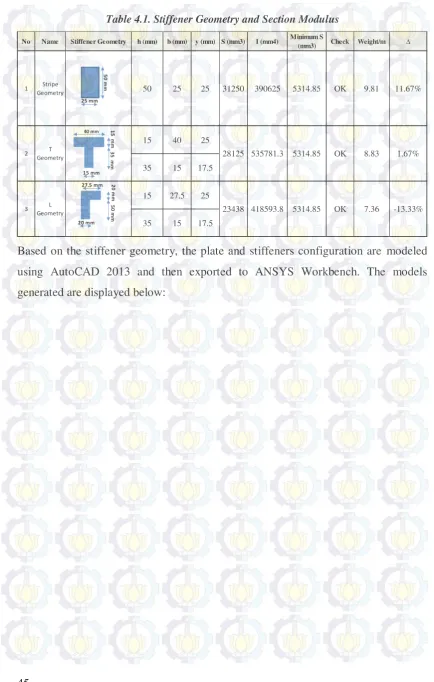
Table 4.1. Stiffener Geometry and Section Modulus
Based on the stiffener geometry, the plate and stiffeners configuration are modeled using AutoCAD 2013 and then exported to ANSYS Workbench. The models generated are displayed below:
No Name Stiffener Geometry h (mm) b (mm) y (mm) S (mm3) I (mm4) Minimum S
(mm3) Check Weight/m ∆
1 Stripe
Geometry 50 25 25 31250 390625 5314.85 OK 9.81 11.67%
15 40 25
3 23438 5314.85 OK 7.36 -13.33%
46
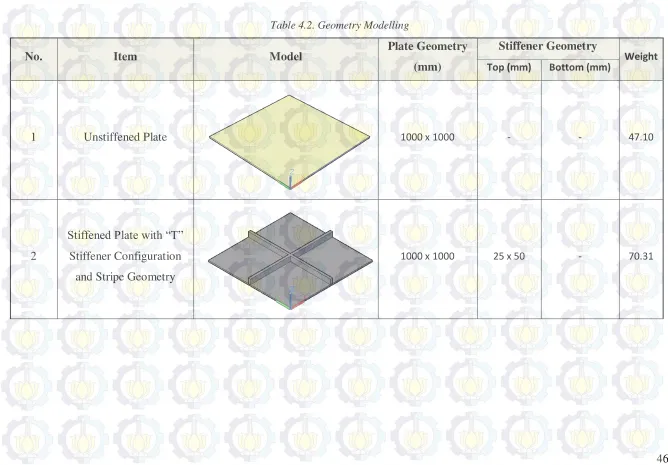
Table 4.2. Geometry Modelling
No. Item Model Plate Geometry
(mm)
Stiffener Geometry
Weight Top (mm) Bottom (mm)
1 Unstiffened Plate 1000 x 1000 - - 47.10
2
Stiffened Plate with “T”
Stiffener Configuration and Stripe Geometry
47
Table 4.2. Geometry Modelling (Continued)
No. Item Model Plate Geometry
(mm) Stiffener Geometry
Weight
3
Stiffened Plate with Parallel Stiffener Configuration and Stripe
Geometry
1000 x 1000 25 x 50 - 70.65
4
Stiffened Plate with “X”
Stiffener Configuration and Stripe Geometry
1000 x 1000 25 x 50 - 79.47
5
Stiffened Plate with “T”
Stiffener Configuration and T Geometry
48
No. Item Model Plate Geometry
(mm) Stiffener Geometry
Weight
6
Stiffened Plate with Parallel Stiffener Configuration and T
Geometry
1000 x 1000 40 x 15 15 x 35 68.30
7
Stiffened Plate with “X”
Stiffener Configuration and T Geometry
1000 x 1000 40 x 15 15 x 35 76.26
8
Stiffened Plate with “T”
Stiffener Configuration and L Geometry
49
Table 4.2. Geometry Modelling (Continued)
No. Item Model Plate Geometry
(mm) Stiffener Geometry
Weight
9
Stiffened Plate with Parallel Stiffener Configuration and L
Geometry
1000 x 1000 27.5 x 15 15 x 35 64.76
10
Stiffened Plate with “X”
Stiffener Configuration and L Geometry
50 The model is then validated compared to hand calculation, prior studies, and meshing sensitivity.
4.1.1.1
Meshing Validation and Sensitivity Study
Upon the sets of models, one model is validated, that is the unstiffened plate with fixed ends. The model is exported to ANSYS Design Modeler (ANSYS DM), and given the mechanical properties as stated in project limitation. The model compared over the model developed by Tavakoli et. al (2012) and by hand calculation that the procedures developed by DNV as stated at equation (6). Meshing sensitivity is also deployed to gain the steady result of modelling and optimum calculation time. The result is as follows:
Table 4.3. Model Validation and Meshing Sensitivity
Meshing (mm) Tn (seconds) Δ (Compared to
The result shows that the optimum meshing size is at 40 mm. Despite the 120 and 80
mm size giving the smaller Δ, the sensitivity graph shows that the natural period
51
Figure 4.1. Meshing Sensitivity Graph
4.1.2
Weight Validation
The weight for each models are calculated to gain the fair analysis comparison, remembering a dynamic analysis is greatly influenced by the mass factor, so that with averagely same mass but higher inertia, stiffener strength will have significant increase. The weight is calculated and compared over the average weight. The deviations for all models are below 15% so the models are approved as valid.
Table 4.4. Weight Calculation and Ratio
NO ITEM WEIGHT
2 Stiffener Parallel Stripe Geometry 70.65 0.36%
3 Stiffened “X” Stripe Geometry 79.47 12.89%
4 Stiffener “T” L Geometry 68.02 -3.38%
5 Stiffened Parallel L Geometry 68.30 -2.99%
6 Stiffened “X” Stiffener L Geometry 76.26 8.33%
7 Stiffened “T” T Geometry 64.47 -8.42%
8 Stiffened Plate Parallel T Geometry 64.76 -8.01%
52
4.1.3
Material Modelling
The material used is ASTM A36 with these following properties:
Table 4.5. Material Properties
No. Properties Value
1. Density 7850 kg/m3
2. Young’s Modulus 200000 MPa 3. Poisson Ratio 0.3
6. Yield Strength 255 MPa 7. Ultimate Strength 400 MPa
Based on DNV OS-C101 LRFD, the yield and ultimate strength (resistance) should
be multiplied by material factor γm, and based on DNV RP-C204, the material resistance curve which is used should be accounted for strain hardening, therefore, the resistance curve is as follow:
Table 4.6. Resistance Curve Table
Strain
Figure 4.2. Factored Resistance Curve
53
4.1.4
Load Modelling
The blast load modelled as uniform pressure subjecting perpendicular to plate front face. The properties of exploded propane gas vapor are as follows:
Table 4.7. Propane Gas Explosion Properties
No. Property Value
1. Density (ρs) 1.24 kg/m3 2. Velocity (vs) 1,660 m/s
The blast duration, as stated at limitation, is varied at 50, 100 and 200 ms. The effect of duration variation is the most important to be accounted for, due to the short-and-heavy load characteristic of blast load, and it is implies the magnitude of impulse generated from the loads. Peak overpressure Ps, which is the maximum pressure at td/2, produced from the drag force calculated from drag force equation (10):
Hence, the peak overpressure Ps = 1,998,912 Pa = 1.99 MPa ≈ 2MPa
The load profile is graphically represented as follows:
54
Configuration and Stripe Geometry 2
50
5 100
6 200
7
Stiffened Plate with Parallel Stiffener Configuration and Stripe Geometry 2
50
8 100
9 200
10
Stiffened Plate with “X” Stiffener
Configuration and Stripe Geometry 2
50
11 100
12 200
13
Stiffened Plate with “T” Stiffener
Configuration and L Geometry 2
50
14 100
15 200
16
Stiffened Plate with Parallel Stiffener Configuration and L Geometry 2
50
17 100
18 200
19
Stiffened Plate with “X” Stiffener
Configuration and L Geometry 2
50
20 100
21 200
22
Stiffened Plate with “T” Stiffener
Configuration and T Geometry 2
50
23 100
24 200
25
Stiffened Plate with Parallel Stiffener Configuration and T Geometry 2
50
26 100
27 200
28
Stiffened Plate with “X” Stiffener Configuration and T Geometry 2
50
29 100
55
4.2
Analysis Result
Analysis is performed based on the analysis matrix. The analysis result for blast duration Td = 50 ms, Td = 100 ms, and Td = 200 ms is as follows:
4.2.1
Modal Analysis
Modal analysis is performed to obtain the 1st order natural period. The results are shown in Table 4.9 below, meanwhile the complete analysis setting and result served in Appendix A:
Table 4.9. Natural Period and Analysis Region
No. Item Natural Period
(s) Td/T Region
1 Unstiffened Plate 0.1891 1.058 Dynamic
2 Config T Geom Stripe 0.0760 2.632 Dynamic
3 Config Parallel Geom
Stripe 0.0812 2.463 Dynamic 4 Config X Geom Stripe 0.0674 2.967 Dynamic
5 Config T Geom L 0.0821 2.436 Dynamic
6 Config Parallel Geom L 0.0715 2.797 Dynamic
7 Config X Geom L 0.0671 2.981 Dynamic
8 Config T Geom T 0.0807 2.478 Dynamic
9 Config Parallel Geom T 0.0798 2.506 Dynamic
56
4.2.2
General Midpoint Deformation Result
The midpoint deformation result for each configuration and blast duration are shown in figure 4.4 to figure 4.6. The maximum values are tabulated in table 4.10. The complete analysis setting and result is displayed at Appendix B.
57
Figure 4.5. Midpoint Deformation 100 ms Blast Duration
58
Table 4.10. Maximum Midpoint Deformation Value
No Plate Midpoint Displacement (mm)
50 ms 100 ms 200 ms
1 UNSTIFFENED PLATE 90.42 93.34 93.50
2 CONFIG T GEOMETRY STRIPE 65.79 65.77 65.69
3 CONFIG PARALLEL GEOM STRIPE 73.11 62.01 60.07
4 CONFIG X GEOMETRY STRIPE 73.26 73.30 75.78
5 CONFIG T GEOMETRY T 60.57 61.74 64.06
6 CONFIG PARALLEL GEOM T 56.90 59.03 59.10
7 CONFIG X GEOMETRY T 62.52 62.80 64.41
8 CONFIG T GEOMETRY L 67.52 68.22 70.22
9 CONFIG PARALLEL GEOM L 59.00 59.22 59.58
10 CONFIG X GEOMETRY L 67.40 67.43 69.72
4.2.3
General Midpoint Von Mises Stress Value
59
Figure 4.7. Midpoint Von Mises Stress 50 ms Blast Duration
61
Table 4.11. Maximum Midpoint Deformation Value
No Plate Midpoint V Mises Stress (MPa)
50 ms 100 ms 200 ms
1 UNSTIFFENED PLATE 348.00 348.00 348.00
2 CONFIG T GEOMETRY STRIPE 347.81 347.66 347.57
3 CONFIG PARALLEL GEOM STRIPE 347.74 347.57 347.32
4 CONFIG X GEOMETRY STRIPE 347.72 347.75 347.77
5 CONFIG T GEOMETRY T 346.56 346.63 346.65
6 CONFIG PARALLEL GEOM T 346.68 346.78 347.12
7 CONFIG X GEOMETRY T 347.79 347.78 347.80
8 CONFIG T GEOMETRY L 347.80 347.72 347.79
9 CONFIG PARALLEL GEOM L 347.74 347.78 348.00
10 CONFIG X GEOMETRY L 347.74 347.87 347.95
4.3
Discussion
Based on the result displayed, there are some effects that interesting to be discussed. Based on the equation (15) to (18), there are some factors to be considered to control
the response of dynamic system. Let’s recall the dynamic equilibrium equation as
stated by equation (15):
𝑚𝑢̈(𝑡) + 𝑏𝑢̇(𝑡) + 𝑘𝑢(𝑡) = 𝑓(𝑡) (15)
Where: