Series Editor
Professor Brian Derby, Professor of Materials Science
Manchester Materials Science Centre, Grosvenor Street, Manchester, M1 7HS, UK
Other titles published in this series
Fusion Bonding of Polymer Composites
C. Ageorges and L. Ye
Composite Materials
D.D.L. Chung
Titanium
G. Lütjering and J.C. Williams
Corrosion of Metals
H. Kaesche
Corrosion and Protection
E. Bardal
Intelligent Macromolecules for Smart Devices
L. Dai
Microstructure of Steels and Cast Irons
M. Durand-Charre
Phase Diagrams and Heterogeneous Equilibria
B. Predel, M. Hoch and M. Pool
Computational Mechanics of Composite Materials
M. Kamiński
Gallium Nitride Processing for Electronics, Sensors and Spintronics
S.J. Pearton, C.R. Abernathy and F. Ren
Materials for Information Technology
E. Zschech, C. Whelan and T. Mikolajick
Fuel Cell Technology
N. Sammes
Casting: An Analytical Approach
A. Reikher and M.R. Barkhudarov
Computational Quantum Mechanics for Materials Engineers
L. Vitos
Modelling of Powder Die Compaction
P.R. Brewin, O. Coube, P. Doremus and J.H. Tweed
Silver Metallization
D. Adams, T.L. Alford and J.W. Mayer
Microbiologically Influenced Corrosion
R. Javaherdashti
Modeling of Metal Forming and Machining Processes
P.M. Dixit and U.S. Dixit
Electromechanical Properties in Composites Based on Ferroelectrics
William W. Sampson
Modelling Stochastic Fibrous
Materials with Mathematica
®
School of Materials University of Manchester Sackville Street
Manchester M60 1QD UK
ISBN 978-1-84800-990-5 e-ISBN 978-1-84800-991-2 DOI 10.1007/978-1-84800-991-2
Engineering Materials and Processes ISSN 1619-0181 A catalogue record for this book is available from the British Library Library of Congress Control Number: 2008934906
© 2009 Springer-Verlag London Limited
Mathematica and the Mathematica logo are registered trademarks of Wolfram Research, Inc. (“WRI” – www.wolfram.com) and are used herein with WRI’s permission. WRI did not participate in the crea-tion of this work beyond the inclusion of the accompanying software, and offers it no endorsement beyond the inclusion of the accompanying software.
Apart from any fair dealing for the purposes of research or private study, or criticism or review, as permitted under the Copyright, Designs and Patents Act 1988, this publication may only be repro-duced, stored or transmitted, in any form or by any means, with the prior permission in writing of the publishers, or in the case of reprographic reproduction in accordance with the terms of licences issued by the Copyright Licensing Agency. Enquiries concerning reproduction outside those terms should be sent to the publishers.
The use of registered names, trademarks, etc. in this publication does not imply, even in the absence of a specific statement, that such names are exempt from the relevant laws and regulations and therefore free for general use.
The publisher makes no representation, express or implied, with regard to the accuracy of the infor-mation contained in this book and cannot accept any legal responsibility or liability for any errors or omissions that may be made.
Cover design: eStudio Calamar S.L., Girona, Spain Printed on acid-free paper
Preface
This is a book with three functions. Primarily, it serves as a treatise on the structure of stochastic fibrous materials with an emphasis on understanding how the properties of fibres influence those of the material. For some of us, the structure of fibrous materials is a topic of interest in its own right, and we shall see that there are many features of the structure that can be characterised by rather elegant mathematical treatments. The interest of most researchers how-ever is the manner in which the structure of fibrous networks influences their performance in some application, such as the ability of a non-woven textile to capture particles in a filtration process or the propensity of cells to proliferate on an electrospun fibrous scaffold in tissue engineering. The second function of this book is therefore to provide a family of mathematical techniques for mod-elling, allowing us to make statements about how different variables influence the structure and properties of materials. The final intended function of this book is to demonstrate how the softwareMathematica1can be used to support the modelling work, making the techniques accessible to non-mathematicians. We proceed by assuming no prior knowledge of any of the main aspects of the approach. Specifically, the text is designed to be accessible to any sci-entist or engineer whatever their experience of stochastic fibrous materials, mathematical modelling or Mathematica. We begin with an introduction to each of these three topics, starting with defining clearly the criteria that clas-sify stochastic fibrous materials. We proceed to consider the reasons for using models to guide our understanding and specifically whyMathematicahas been chosen as a computational aid to the process.
Importantly, this book is intended not just to be read, but to beused. It has been written in a style intended to allow the reader to extract all the impor-tant relationships from the models presented without using theMathematica
1 A trial version of Mathematica 6.0 can be downloaded from
examples provided. However, for a comprehensive understanding of the science underlying the models, readers will benefit from running the code and editing it to probe further the dependencies we identify and discuss. TheMathematica code embedded in the text includes numbers added byMathematicaon eval-uation. Where a line of code begins with ‘In[1]:=’ this indicates that a new session on the Mathematica kernel has been started and previously defined variables,etc.no longer exist in the system memory.
When preparing the manuscript, some consideration was given as to the appropriate amount ofMathematicacode to include. In common with many scientists, the author’s first approach to any theoretical analysis involves the traditional tools of paper and pencil, with the use ofMathematicabeing intro-duced after the initial formulation of the problem of interest. Typically how-ever, once progress has been made on a problem, the early manipulations,etc. are subsequently entered intoMathematicaso that the full treatment is con-tained in a single file. As a rule, we seek to replicate this approach by providing many of the preliminary relationships and straightforward manipulations as ordinary typeset equations before turning to Mathematicafor the more de-manding aspects of the analysis. Occasionally, where the outputs of relatively simple manipulations are required for subsequent treatments,Mathematicais invoked at an earlier stage.
Consideration was given also as to whether to includeMathematica code for the generation of plots, or to provide these only in the form of figures with supplementary detail, such as arrows,etc.One of the great advantages of work-ing with Mathematica is that its advanced graphics capabilities allow rapid generation of plots and surfaces representing functions; surfaces can be rotated using a mouse or other input device and dynamic plots with interactivity are readily generated. When developing theory, the ability to visualise functions guides the process and can provide valuable reassurance that functions behave in a way that is representative of the physical system of interest. Accordingly, theMathematicacode used to generate graphics is provided in the majority of instances and graphics are not associated with figure numbers, but instead are shown as the output of a Mathematica evaluation. Where graphics are associated with a figure number, the content is either a drawing to guide our analysis or a collection of results from severalMathematicaevaluations; in the latter case, plots or surfaces have been typically generated usingMathematica and exported to graphics software for the addition of supplementary detail and annotation.
outcomes from our fifteen years of fruitful and enjoyable research collaboration are included in this monograph.
Thanks are also due to Maryka Baraka of Wolfram Research for support and advice, to Steve Eichhorn for permission to reproduce the micrograph of an electrospun nanofibrous network in Figure 1.1 and to Steve Keller for permission to reproduce Figures 5.7 and 5.8. I would like to thank Taylor and Francis Ltd. for permission to reproduce Figure 3.7, Journal of Pulp and Paper Science for permission to reproduce Figure 6.1 and Wiley-VCH Verlag GmbH & Co. KGaA for permission to reproduce Figure 7.1.
Manchester Bill Sampson
Contents
1 Introduction. . . 1
1.1 Random, Near-Random and Stochastic . . . 3
1.2 Reasons for Theoretical Analysis . . . 9
1.3 Modelling withMathematica. . . 11
2 Statistical Tools and Terminology. . . 15
2.1 Introduction . . . 15
2.2 Discrete and Continuous Random Variables . . . 15
2.2.1 Characterising Statistics . . . 16
2.3 Common Probability Functions . . . 29
2.3.1 Bernoulli Distribution . . . 29
2.3.2 Binomial Distribution . . . 31
2.3.3 Poisson Distribution . . . 35
2.4 Common Probability Density Functions . . . 37
2.4.1 Uniform Distribution . . . 38
2.4.2 Normal Distribution . . . 39
2.4.3 Lognormal Distribution . . . 42
2.4.4 Exponential distribution . . . 45
2.4.5 Gamma Distribution . . . 46
2.5 Multivariate Distributions . . . 49
2.5.1 Bivariate Normal Distribution . . . 51
3 Planar Poisson Point and Line Processes . . . 55
3.1 Introduction . . . 55
3.2 Point Poisson Processes . . . 55
3.2.1 Clustering . . . 56
3.2.2 Separation of Pairs of Points . . . 63
3.3 Poisson Line Processes . . . 71
3.3.1 Process Intensity . . . 73
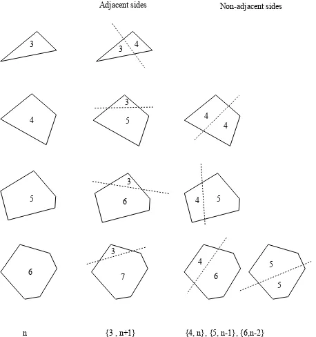
3.3.3 Statistics of Polygons . . . 83
3.3.4 Intrinsic Correlation . . . 94
4 Poisson Fibre Processes I: Fibre Phase . . . 105
4.1 Introduction . . . 105
4.2 Planar Fibre Networks . . . 105
4.2.1 Probability of Crossing . . . 110
4.2.2 Fractional Contact Area . . . 115
4.2.3 Fractional Between-zones Variance . . . 117
4.3 Layered Fibre Networks . . . 132
4.3.1 Fractional Contact Area . . . 132
4.3.2 In-plane Distribution of Fractional Contact Area . . . 137
4.3.3 Intensity of Contacts . . . 146
4.3.4 Absolute Contact States . . . 150
5 Poisson Fibre Processes II: Void Phase . . . 159
5.1 Introduction . . . 159
5.2 In-plane Pore Dimensions . . . 160
5.3 Out-of-plane Pore Dimensions . . . 171
5.4 Porous Anisotropy . . . 174
5.5 Tortuosity . . . 182
5.6 Distribution of Porosity . . . 184
5.6.1 Bivariate Normal Distribution . . . 185
5.6.2 Implications for Network Permeability . . . 191
6 Stochastic Departures from Randomness . . . 195
6.1 Introduction . . . 195
6.2 Fibre Orientation Distributions . . . 196
6.2.1 One-parameter Cosine Distribution . . . 196
6.2.2 von Mises Distribution . . . 199
6.2.3 Wrapped Cauchy Distribution . . . 201
6.2.4 Comparing Orientation Distribution Functions . . . 202
6.2.5 Fibre Crossings . . . 206
6.2.6 Crossing Area Distribution . . . 211
6.2.7 Mass Distribution . . . 216
6.3 Fibre Clumping and Dispersion . . . 217
6.3.1 Influence on Network Parameters . . . 222
7 Three-dimensional Networks. . . 241
7.1 Introduction . . . 241
7.2 Network Density . . . 244
7.2.1 Crowding Number . . . 246
7.3 Intensity of Contacts . . . 248
7.5 Variance of Areal Density . . . 253
7.6 Sphere Caging . . . 258
References. . . 265
1
Introduction
Probably the oldest and most familiar stochastic fibrous material to most of us is that on which this text is printed. Tradition has it that paper was invented in China at the start of the second century CE though there is some evidence for its existence as early as the second century BCE. Regardless of the precise date that paper saw its first use, we may be confident that it is not as old as the material from which it takes its name, papyrus. These two materials, both of which have been so important in recording the development of society and ideas, provide a good pair of examples with which we can guide our classification of materials as stochastic. Papyrus is made from the pithy inner part of the stem of the sedgeCyperus papyrus; during the manufacture of papyrus, this is cut into long strips that are laid side by side on a flat surface with their edges overlapping. A second layer with the strips oriented perpendicularly to those in the first layer is placed over the first. On drying, these strips bond to each other to yield the sheet-like material we call papyrus. So, during the manufacture of papyrus, each strip is carefully placed in relation to those strips which have already been laid down and, given knowledge of the location and orientation of one strip, we can be quite confident of the location and orientation of others. This regularity in the structure classifies it as deterministicand other materials with structures encompassed by this classification include woven textiles, honeycomb structures,etc.
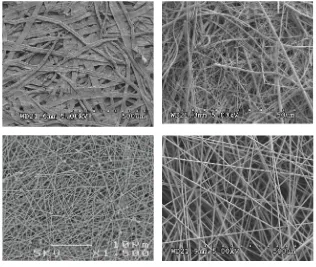
Figure 1.1.Micrographs of four planar stochastic fibrous materials. Clockwise from top left: paper formed from softwood fibres, glass fibre filter, non-woven carbon fibre mat, electrospun nylon nanofibrous network (Courtesy S.J. Eichhorn and D.J. Scurr. Reproduced with permission)
to make statements of theprobabilityof a given structural feature occurring, the material is neither uniform nor regularly non-uniform, but it is variable in a way that can be characterised by statistics. Accordingly, we classify paper and similar materials asstochastic.
the fibres, the distances between adjacent intersections on any given fibre are sufficiently close that the fibrous ligaments between these can be considered, to a reasonable approximation, as being straight so the inter-fibre voids are rather polygonal.
Two networks formed from very straight fibres are shown on the bottom of Figure 1.1. The image on the right shows a network of carbon fibres used in electromagnetic shielding applications and in the manufacture of gas diffusion layers for use in fuel cells. In common with paper and the glass fibre filter that we have just considered, this material is formed by a process where fibres are deposited from an aqueous suspension. The micrograph reveals another important structural property of the planar stochastic fibrous materials that we have considered so far – the fibres lie very much in the plane of the network and do not exhibit any significant degree of entanglement. We shall consider this further in the sequel, and will utilise this property of materials in de-veloping models characterising their structures. The network on the bottom left of Figure 1.1 shares these characteristics though it is formed by a very different process: electrospinning. Here the fibres from which the network is formed are manufactured in the same process as the network itself and as the filament leaves the spinneret it is subjected to electrostatic forces, elongating it and yielding a layered stochastic fibrous network. There has been consider-able interest in such materials in recent years, driven in part by the potential of electrospinning processes to yield fibres of width a few nanometres and fi-bres that are themselves porous, providing opportunities to tailor structures for application as biomaterials and for nanocomposite reinforcements, seee.g. [91].
In Chapters 3 to 6 we will derive models for materials of the type we have discussed so far, where fibre axes can be considered to lie in the plane of the material. These layered structures represent the most common type of fibre network encountered in a range of technical and engineering applications. Stochastic fibrous materials do exist however where fibre axes are oriented in three dimensions. These include needled and hydro-entangled non-woven textiles such as felts and insulating materials and the fibrous architectures within short-fibre reinforced composite materials. We derive models for the structure of this class of materials in Chapter 7.
1.1 Random, Near-Random and Stochastic
were identified in one of the seminal works on modelling planar random fibre networks, that of Kallmes and Corte [74]. These are:
• the fibres are deposited independently of one another;
• the fibres have an equal probability of landing at all points in the network;
• the fibres have an equal probability of making all possible angles with any arbitrarily chosen, fixed axis.
So, from the first two of these criteria, we consider the random events to be the incidence of fibre centres within an area that represents some or all of our network. Now, fibre centres exist at points in space, but the third criterion given by Kallmes and Corte arises because fibres are extended objects, i.e. they have appreciable aspect ratio. In their simplest form, we may consider fibres as rectangles with their major axes being straight lines. The third crite-rion tells us that these major axes have equal probability of lying within any interval of angles, so it effectively restates the first two criteria for lines rather than points—the angle made by the major axis of a fibre is independent of those of other fibres and all angles are equally likely. When fibres are not straight but exhibit some curvature along their length, then the same defi-nition holds, but for the third criterion we consider that the tangents to the major axis have an equal probability of making all possible angles with any arbitrarily chosen, fixed axis. Note that for materials such as those shown in Figure 1.1 we consider orientation of fibre axes to be effectively in the plane, whereas for three-dimensional networks, orientation is defined by solid angles in the range 0 to 2πsteradians. Tomographic images of networks of this type are shown in Figure 7.1.
Graphical representations of random point and line processes generated using Mathematicaare shown in Figure 1.2. The graphic on the left of Fig-ure 1.2 shows 1,000 points which we will consider to represent the centres of fibres. These points are generated independently of each other with equal probability that they lie within any region of the unit square. On first in-spection, we note a very important property of random processes—they are not regularly spaced but are clustered,i.e.they exhibit clumping. The extent of this clustering is a characteristic of the process that depends upon its in-tensity only, so for our process of fibre centres in the unit square it depends upon the number of fibre centres per unit area. The graphic on the right of Figure 1.2 uses the coordinates of the points shown in the graphic on the left as the centres of lines with length 0.1 and with uniformly random orientation as stipulated in the third criterion of Kallmes and Corte. The interaction of lines with each other provides connectivity to the network and increases our perception of its non-uniformity through, for example, the intensity of the line process within different regions of the unit square or the different sizes of polygons bounded by these lines in the same regions.
Figure 1.2. Random point and fibre processes in two dimensions. Left: 1,000 ran-dom points in a unit square; right: the same points extended to be ranran-dom lines with the points at their centre and with length 0.1
now we state simply that a random fibre process is a specific class of pro-cess that exactly satisfies the criteria of Kallmes and Corte mathematically. When networks are made in the laboratory or in an industrial manufactur-ing context, the resultant structures typically display some differences from those generated by model random processes, i.e. system influences combine to yield networks with structures that are manifestly not deterministic, so we still require the use of statistics to describe them, yet also they do not meet the precise mathematical criteria that permit them to be classified as random. We will characterise such influences as yielding ‘departures from randomness’,
and these fall into three principal categories:
• Preferential orientation of fibres to a given direction,
• Fibre clumping,
• Fibre dispersion.
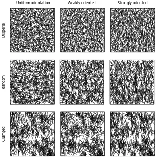
Graphical representations of these departures from randomness are given in Figure 1.3 for networks of 1,000 lines of uniform length 0.1 with centres oc-curring within a unit square. The structure on the left of the second row represents a model random network.
R
andom
Clumped
Disperse
Uniform orientation Weakly oriented Strongly oriented
Figure 1.3. Departures from randomness. Industrially formed networks typically exhibit different degrees of fibre clustering and fibre orientation than the model random fibre network shown on the left of the second row
A B C
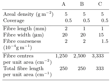
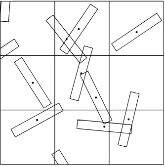
Figure 1.4. Influence of fibre properties on structures of random fibre networks. Graphic rendered to allow fibre length to extend beyond the square region containing fibre centres
Whereas a preferential orientation of fibres in a network is potentially rather easy to observe, the extent of clumping or dispersion in the network is not so readily detected. In part this is because the extent of clumping in a network depends upon the geometry and morphology of its constituent fibres. We illustrate this in Figure 1.4, which shows three simulated random networks of straight uniform fibres; each network has mass per unit area, 5 g m−2 and consists of fibre centres occurring as a uniform random process in a square of side 1 cm. The mass per unit area of fibrous materials is often termed thegrammageof the network, or itsareal density. Three properties of fibres were required to generate the structures shown in Figure 1.4: the length and width of fibres and their mass per unit length; this property of fibres is termed coarseness or linear density and is often reported for textiles and textile filaments in units of denier, or grams per 9,000 metres. The fibre and network properties for the networks shown in Figure 1.4 are given in Table 1.1, which introduces also the network variable coverage, which we define as the number of fibres covering a point in the plane of support of the network; the average coverage of the network is given by its mass per unit area divided by that of the constituent fibres. Since the coarseness of a fibre is defined as its mass per unit length, it follows that its mass per unit area is given by its coarseness divided by its width, so the coverage is given by
Coverage = Network areal density×Fibre width
Fibre coarseness .
Table 1.1. Fibre and network properties for networks shown in Figure 1.4
A B C
Areal density (g m−2) 5 5 5
Coverage 0.5 0.5 0.5
Fibre length (mm) 2 1 1
Fibre width (μm) 20 20 15
Fibre coarseness 2 2 1.5
(10−4g m−1)
Fibre centres 1,250 2,500 3,333
per unit area (cm−2)
Total fibre length 250 250 333
per unit area (cm−1)
the uniformity of the networks improves as we move from left to right. Re-ferring to Table 1.1 we note that the fibres in Network A are twice as long as those in Network B. Thus, to achieve the same areal density and coverage, Network B consists of twice as many fibres as Network A. Accordingly, the total fibre length per unit area in Networks A and B is the same, yet their structures differ through the number of fibres per unit area and the extent of interaction of a given fibre with others in the network; we expect the latter to be a function of fibre length. Similarly, Network C exhibits greater unifor-mity than Network B because it has greater fibre length per unit area as a consequence of the linear density of the constituent fibres being less.
charac-terise the full family of fibrous networks governed by spatial distributions of fibres with a distribution of orientations as ‘stochastic’; the term ‘random’ is used for model structures the conform to the criteria of Corte and Kallmes, as introduced on page 4. Where departures from randomness are weak, we will classify our structures as ‘near-random’. No strict demarcations exist between these terms, and we shall see that whilst some properties of a given stochastic material may differ significantly from the random case, in the same sample others may be remarkably close.
1.2 Reasons for Theoretical Analysis
Before looking at the reasons for using Mathematicato assist the modelling process, it is worth considering why modellingper seis a useful tool when ap-plying the scientific method. A good mathematical model provides expressions that describe the behaviour of a system faithfully in terms of the variables that influence it. A good example of such a model is the equation for the period,T (s) of a simple pendulum, which most of us have encountered:
T = 2π
l
g , (1.1)
wherel(m) is the length of the pendulum from its pivot point to the centre of mass of the bob andg(m s−2) is the acceleration due to gravity. The derivation of Equation 1.1 depends on some assumptions:
• the bob is a point mass;
• the string or rod on which the bob swings has no mass;
• the motion of the pendulum occurs in a plane;
• the pendulum exists in a vacuum;
• the initial angle of the string or rod to the vertical, θ, is sufficiently small that θ≈sin(θ).
the assumptions made in deriving Equation 1.1 do not apply, then we must use a more complicated model, and probably must work a little harder to make good predictions of its behaviour.
Of course, Equation 1.1 is a simple expression describing a simple sys-tem. Indeed, by conducting a series of experiments measuring the periods of pendulums with different weight bobs, string lengths and initial angular dis-placements, it is likely that after some informed data processing we might come up with a similar equation by heuristic methods. Such experiments are useful to theoreticians in their own right – they provide data against which we can compare our theories in order that we can verify them, or, if agreement is not as good as we would like, the differences guide the development of more faithful models – they are, however, time consuming and most systems are significantly more complex than the simple pendulum.
Now, there is uncertainty associated with any experimental measurement and we might characterise this by reporting the spread of experimental data about the mean using, for example, confidence intervals. For a determinis-tic process, such as the swinging of a simple pendulum, the spread of data captures variability due to experimental error, instrument accuracy,etc.The materials of interest to us are stochastic and, by definition, there is additional variability in measurements of their properties that is not due to experimental error or uncertainty, but which is a characteristic of the material. Accordingly, we will seek to model the likelihood that the networks exhibit certain proper-ties and, for the properproper-ties that exhibit dependence on many variables, theory allows us to identify which of these have the more significant influence on the property of interest. In stochastic fibre networks we do not know the location or orientation of any individual component such as a fibre, pore or inter-fibre contact, relative to others in the structure. We must therefore use statistics to describe their combined effect and, provided the number of components is sufficiently large, theory will accurately describe the properties of the network as a whole.
As well as guiding practical work and our thinking, theory can be used to provide insights which are rather difficult to obtain even in the controlled environment of the laboratory. Consider the linear density of fibres, which we encountered on page 7 and defined as their mass per unit length. A fibre of circular cross section with widthω and density,ρ, has linear density given by
δ=π ω
2
4 ρ . (1.2)
So we see that linear density is proportional to the square of fibre width such that if we alter fibre width in an experimental setting, then we expect to in-fluence linear density also. Thus we would be unable to determine without further experimentation whether an observed behaviour is due to the change in width or the change in linear density. Of course, we might carry out ex-periments using hollow fibres, where changing the thickness of the fibre wall allows us to change fibre width without changing linear density. Obtaining such fibres, with sufficiently well characterised geometries may prove rather difficult, but the experiment could be carried out. Using a theoretical ap-proach however, we can include fibre width and linear density asindependent variables in a model, so that their influence on the property of interest can be decoupled. Accordingly, models conserve and focus experimental effort.
The final reason for theoretical analysis that we consider here is that equa-tions enable us to model systems outside the realms permitted by experiments. Thus, whilst it may be difficult to obtain an experimental measure of, for ex-ample, the tortuosity of paths from one side of a fibre network to the another, an expression for this property is rather easy to derive for an isotropically porous material (cf. Section 5.5). In short, our models should represent ap-plied mathematics in a form that is both useful and useable. Throughout the following chapters, we seek to simplify our analyses to provide accessible and tractable expressions aiding their application.
1.3 Modelling with
Mathematica
Mathematicaserves as rather a good teacher also. Consider, for example, the integral
ex
x dx .
We input this intoMathematicaas
In[1] = Integratexx, x
where the second argument of the command Integrate specifies that we want to integrate our function with respect to x. We press Shift + Enter
together to evaluate our input and obtain the output:
Out[1]= ExpIntegralEix
By selecting this output and pressing the F1 key, we access theMathematica help files for ExpIntegralEi we identify the function as the exponential integral function. This is an example of a ‘special function’ that few of us other than mathematicians will have encountered in formal studies. We will encounter it later, but what is important for now is the fact thatMathematica will handle most functions that we present to it and that it may provide us with answers with which we are unfamiliar. Importantly, through the help files and exploration of these functions we rapidly become familiar with them. So we may do, for example,
In[2]:= PlotExpIntegralEix,x, 2, 2
Out[2]=
2 1 1 2
6 4 2 2 4
In fact, we could ask Mathematica to carry out the same integral using several different notations. For example,
In[3]:= IntegrateExpx x, x
In[4]:= x
x
x
In[5]:= IntegrateE ^ xx, x
are all equivalent. This is important. Different users prefer different styles of in-put; accordingly, the code presented in the chapters that follow represents just one way of approaching the problems we consider. Mathematica has a large array of palettes allowing symbolic input of expressions such that they closely resemble what we write with a pencil and paper. Typically, theMathematica code presented here will have been composed with commands given as words rather than as symbols, so we shall useIntegrateinstead of
,Suminstead of ,
etc. Regardless of the chosen style of input, the computation will be symbolic, rather than numerical, unless stated otherwise.
In addition to its strong symbolic capabilities, Mathematica provides an excellent environment for experimental mathematics. In particular, the
com-mandManipulateprovides interactivity which can guide our thinking. We
illustrate this by considering a simple example where we investigate the range ofxfor which the approximation sin(x)≈xis reasonable. In our example, the first argument of theManipulatecommand specifies the function of inter-est; the second argument specifies that we seek to vary parameterxbetween 0 andπwith starting valuex= 1:
In[6]:= Manipulatex, Sinx x, x, 1., 0, Π
Out[6]=
x
1., 0.841471
The output includes a slider that can be used to vary the value of parameterx and yield the bracketed term{x,sin(x)/x} in the output field.
by applying the rule-of-thumb that dynamic objects may often be created by replacing the commandTablewith Manipulate.
2
Statistical Tools and Terminology
2.1 Introduction
Having classified our materials as being stochastic, we require a family of mathematical tools to represent the distributions of their properties and some suitable numbers to describe these distributions. This chapter provides infor-mally some background to these tools. A real number is called a ‘random variable’ if its value is governed by a well-defined statistical distribution. We begin by defining some general properties of random variables and many of the distributions that we will encounter in subsequent chapters and that we shall use to derive the properties of stochastic fibrous materials. As well as using standard mathematical notation, the use ofMathematicato handle statistical functions and generate random data is introduced.
2.2 Discrete and Continuous Random Variables
unable therefore to deterministically predict the outcome of a roll and must always be uncertain of any individual event. Despite this uncertainty, we may be confident that the probability of rolling any number is 16. Thus, whereas we cannot predict the outcome of an individual roll, we know what all the possible outcomes are and the probability of their occurrence. We can state then the random variablexwhich represents the outcome of the roll of a die can take the values 1, 2, 3, 4, 5 and 6 and each outcome has probability 1
6. In the sequel, we shall see that this characterises the random variablexas being controlled by the discrete uniform probability distribution,P(x) =1
6. We consider first the application of statistics to the description of systems where the events within that system or the outcomes of it arediscrete. This means that each possible event or outcome has a definite probability of occur-rence. We have just considered one such process, the rolling of an unbiased die. Another example of a discrete stochastic process is the tossing of a coin where the probability of the outcome being either heads or tails is 12. If we assume that the probability of the die coming to rest on one of its edges is infinitesi-mal, then we may state that the probability of each event is 16. Similarly, we know that it is not possible to throw the die and have the uppermost face show, for example, 41
2 spots. So the outcome of rolling the die is a discrete random variable. Examples of discrete random variables that characterise the structure of fibre networks are the number of fibre centres per unit volume or area in the network, or the number of fibres making contact with any given fibre in the structure. As a rule, we can expect to encounter discrete random variables when the feature of interest, experimental conditions permitting, may be counted; the exception to this being where only certain classes of events exist, for example, where a fibre network is formed from a blend of fibres manufactured with precisely known lengths which are known because they have been measured and not because they have been counted.
Consider now the distribution of the weights of eggs produced by free-range hens. The probability that an egg weighs precisely 60 g is very small; as is the probability that it weighs precisely 59.9 g or 60.000001 g. It is much easier, and certainly more meaningful, to state the probability that eggs from these hens weigh between say 55 and 65 g or between 45 and 55 g,etc.Clearly, the weights of the eggs differ from the rolling of a die in that we do not have discrete outcomes; the weight of an egg is therefore classified as acontinuous random variable. Examples of continuous random variables encountered in the description of fibre networks are the area or volume of inter-fibre voids and the lengths of the fibrous ligaments that exist between fibre crossings.
2.2.1 Characterising Statistics
most of us through the handling of experimental data. We define them here for completeness.
Mean: The mean value of the sample data is given by the sum of all the data divided by the number of observations. For data x1, x2. . . xn we denote
The mean is often termed the expectationor, in every-day language, the average.
Mode: The mode is the value within our sample data that occurs with the greatest frequency. For discrete data, this is found by inspection; for con-tinuous data the mode is estimated from a histogram of the data as the mid point of the tallest column.
Median: The median is occasionally used instead of the mean for the charac-terisation of data that has a histogram that is not symmetric about the mean; such data is described as skewed. The median is found by sorting the data by magnitude and selecting the middle observation such that half the observations are numerically greater than the median and half are numerically smaller.
Variance: The variance of our data is the mean square difference from the mean, i.e. it is the expected value of (xi−x)¯ 2. It is denoted σ2(x) and
For small samples of data, Equation 2.2 will underestimate the variance because, for a sample of size n, each observation can be independently compared with only (n−1) other observations, biasing the calculation of the variance. Accordingly, the unbiased estimate of the variance is given by
and this is typically applied for samples with nless than about 20. Standard Deviation: The standard deviation is the square root of the variance
and it is denoted σ(x). It is often preferred to the variance as it has the same units as the original data.
The unbiased estimate is given by
σ(x) =σ2(x) =
n
i=1
(xi−x)¯ 2
n−1 . (2.5)
Coefficient of Variation: The coefficient of variation is the standard deviation relative to the mean. We denote itCV(x) and it is given by
CV(x) =σ(x) ¯
x . (2.6)
Note that the coefficient of variation is dimensionless and is often reported as a percentage.
We classify the mean, mode and median as measures of location; they pro-vide a measure of the magnitude of the numbers we can expect to characterise our distribution. The variance, standard deviation and coefficient of variation are classified as measures of spread; they provide a measure of how widely distributed the data are in our sample or population and thus can be used to inform how representative our measures of location are of the distribution as a whole.
Using Characterising Statistics
We illustrate the calculation of these characterising statistics withMathematica by generating a sample of data representing rolls of a pair of unbiased dice us-ing the command RandomInteger. This function generates pseudorandom integers with equal probability, so the commandRandomInteger[]will give an output of either 0 or 1 with the probability of each outcome being 1
2. To represent the roll of a fair six-sided die we useRandomInteger[1,6].
Consider first the outcomes of rolling a pair of unbiased dice 20 times. The outcomes of the experiment are recorded in the following graphic:
In fact, these dice rolls were simulated inMathematicausingRandomInteger with the following input:
SeedRandom1
which gives the output in list form which corresponds to our graphic:
Out[2]= 5, 3,5, 1,2, 1,1, 3,1, 1,4, 6,3, 1,
4, 5,5, 2,4, 4,5, 2,5, 3,2, 2,5, 6,
5, 6,1, 4,4, 1,1, 3,4, 2,2, 4
Note the use of the commandSeedRandom. By including this line,Mathematica uses the same random seed for each evaluation and we obtain the same value
forpairseach time we evaluate the code. Each pair of numbers is identified
in Mathematicaby its location in the list, so we can refer to these using the commandPartor the assignment[[ ]],e.g.,
In[3] = Partpairs, 4
pairs8
Out[3]= 1, 3
Out[4]= 4, 5
The values obtained by summing the numbers shown on each pair of dice rep-resent the random variable of interest. For the ith pair of random numbers, we obtain their sum usingTotal[pairs[[i]]], and we use the command
Tableto carry this out for alli:
In[5] = rolls TableTotalpairsi, i, 1, 20
Out[5]= 8, 6, 3, 4, 2, 10, 4, 9, 7, 8, 7, 8, 4, 11, 11, 5, 5, 4, 6, 6
To compute the mean of our dice rolls we need to apply Equation 2.1 and compute the sum of all observations and divide this by the number of observa-tions.Mathematicahas a built-in commandMeanto carry out this calculation:
In[6] = Meanrolls
Out[6]= 32
5
The result is displayed as an improper fraction, becauseMathematicahas car-ried out computations on random integers. To convert to the corresponding numerical value, we useN:
In[7] = N
where the symbol % refers to the last output. To compute the variance we require the mean square difference from the mean, as given by Equation 2.3. We might compute this explicitly using,
In[8] = Totalrolls Meanrolls ^ 2 19 N
Out[8]= 644
95
Out[9]= 6.77895
though again,Mathematica has the specific command Variance to handle this for us:
In[10] = Variancerolls
Out[10]= 644
95
Inevitably, the standard deviation is given by,
In[11]:= StandardDeviationrolls N
Out[11]= 2 161
95
Out[12]= 2.60364
and is the square root of the variance:
In[13] = TrueQStandardDeviationrolls Variancerolls
Out[13]= True
Importantly in Version 6,Mathematicaalways uses Equations 2.3 and 2.5 to calculate the variance and standard deviation when handling lists. Note that to generate the square root operator inMathematicawe use Ctrl+2, though
SqrtVariancerolls Variancerolls^12 Variancerolls12
PowerVariancerolls, 12
where in the third example, the superscript is generated using Ctrl+6.
For completeness, we calculate the remaining measures of location and spread for our data, as given earlier in this section:
In[14] = Medianrolls
Commonestrolls Commonest mode
CVrolls StandardDeviationrolls Meanrolls NCVrolls
Out[14]= 6
Out[15]= 4
Out[16]=
805 19
16
Out[17]= 0.406819
The use of the command Median is an intuitive choice, but we note that the command Mode is used in Mathematicain conjunction with commands associated with equation solving and other operations; thus we compute the mode using the commandCommonest. Note that the output of this command is a list enclosed in braces,{ }, in our case this list has length 1, though this need not be the case. Note also the use of the comment enclosed between starred brackets,(* *); anything between these characters is not evaluated. If we change the first line of our code to SeedRandom[2] we obtain a different set of observations:
In[18] = SeedRandom2
pairs RandomInteger1, 6, 20, 2
rolls TableTotalpairsi, i, 1, 20; Out[19]= 6, 2,3, 3,6, 3,2, 6,6, 1,1, 5,4, 5,
1, 2,2, 6,2, 6,5, 5,1, 1,5, 5,2, 3,
4, 4,1, 2,1, 5,3, 3,2, 6,5, 4
In[21] = NMeanrolls NVariancerolls
NStandardDeviationrolls
Out[21]= 6.95
Out[22]= 5.31316
Out[23]= 2.30503
On first inspection, it is clear that the calculated mean, variance and stan-dard deviation for our two sets of simulated dice rolls are different. This arises because we have only a limited set of data available to characterise the dis-tribution, i.e. we are considering the statistics of two samples that we hope are representative of thepopulation from which they are drawn. Using differ-ent values ofSeedRandomwe have generated independent samples from the population of dice rolls where the probabilities of a given number being shown on the face of each dice are equal. Of course, we might pool the results of our two samples to provide a better estimate of the statistics that characterise the distribution:
In[24]:= SeedRandom1
pairs RandomInteger1, 6, 20, 2;
rolls1 TableTotalpairsi, i, 1, 20; SeedRandom2
pairs RandomInteger1, 6, 20, 2;
rolls2 TableTotalpairsi, i, 1, 20; pooledrolls Joinrolls1, rolls2;
Note here that the name pairs is used twice, so values arising from the first evaluation are overwritten in theMathematicakernel by those from the second evaluation. The commandJoin concatenates the specified lists. The characterising statistics for the pooled data are given in the usual way:
In[31] = Lengthpooledrolls NMeanpooledrolls NVariancepooledrolls
NStandardDeviationpooledrolls
Out[31]= 40
Out[32]= 6.675
Out[33]= 5.96859
and we observe that our new estimate of the mean is precisely the mean of our two estimates from the independent samples. The estimates of the variance, and hence the standard deviation, lie between those of the two samples, but are not the mean of these estimates as they are calculated on the basis of the new estimate of the mean and a larger sample withn= 40.
Mathematicacan handle very large lists very comfortably, so we get a much improved estimate of the characterising statistics using largern:
In[35] = SeedRandom1 n 1 000 000;
pairs RandomInteger1, 6, n, 2; rolls
TableTotalpairsi, i, 1, Lengthpairs; MeanNrolls
StandardDeviationNrolls
Out[39]= 7.00089
Out[40]= 2.41501
Note the placing of the commandNsuch that the calculations are performed on numerical rather than integer values of the random variable. This speeds up the calculations as illustrated by use of the command Timing, which gives the output as a list where the first term is the time taken in seconds for Mathematicato perform the calculation:
In[41] = StandardDeviationrolls Timing NStandardDeviationrolls Timing StandardDeviationNrolls Timing
Out[41]= 7.1,
3 375 016 153
37 037
125
Out[42]= 8.142, 2.41501
Out[43]= 0.09, 2.41501
So for this example, the calculation of the standard deviation is almost 80 times faster when performed numerically.
where the first element is the size of the sample,nand the second element is the mean of that sample. UsingListPlotwe are able to visualise the quality of our estimate of the mean as we increase the sample size.
In[44] = meanrollsn Tablen, MeanNTakerolls, n, n, 100, 100 000, 100;
ListPlotmeanrollsn, PlotRangeAll, AxesLabel"n", "Mean"
Out[45]=
20 000 40 000 60 000 80 000 100 000n 6.95
7.00 7.05
Mean
We use similar code to calculate the standard deviation for differentn:
In[46] = stdrollsn
Tablen, StandardDeviationNTakerolls, n, n, 100, 100 000, 100;
ListPlotstdrollsn, PlotRangeAll, AxesLabel"n", "Standard deviation"
Out[47]=
20 000 40 000 60 000 80 000 100 000n 2.40
2.42 2.44 2.46 2.48 Standard deviation
provide us with a reasonable estimate of the characterising statistics for our distribution. When dealing with a sample of size 1 million, we might consider that the statistics of our sample approach those of the population. As yet, though, we do not know precisely the characterising statistics for the popu-lation from which our samples are drawn. Referring back to our simupopu-lation of 1 million rolls, we might reasonably assume that the mean of the popu-lation is 7 and the standard deviation is about 2.42. Note that if we used
SeedRandom[2]to simulate a million rolls of a pair of dice, our estimate of
the mean would change in the 4th decimal place, whereas that of the stan-dard deviation would differ in the third. We will now consider how we can use probability theory to obtain robust measures of location and spread for statistical populations.
Theoretical Determination of Characterising Statistics
Numerical approaches of the type used so far are often referred to as Monte Carlo methods and are very useful when theoretical approaches do not lend themselves to closed form solutions. Very often however, statistical theory does allow us to make precise statements about the properties of distributions. We consider first theory describing the problem of rolling a single die and proceed to consider the case of rolling a pair of dice, which we have just considered.
Consider first the rolling of a fair six-sided die. The only possible out-comes are the integers 1 to 6 and each outcome has probability 16. Since the family of possible outcomes is limited to these values, we have a discrete random variable and, since all outcomes have the same probability, our ran-dom variable has adiscrete uniform distribution. For random integersxwith xmin≤x≤xmax the probability of a givenxi is given by
P(x) = ⎧ ⎨
⎩
0 ifx < xmin
1
1+xmax−xmin ifxmin≤x≤xmax
0 otherwise
(2.7)
InMathematicathe discrete uniform distribution is input as
In[1] = DiscreteUniformDistributionxmin, xmax
Out[1]= DiscreteUniformDistributionxmin, xmax
and the probability function is input using
In[2] = PDFDiscreteUniformDistributionxmin, xmax, x
Out[2]=
1
which corresponds to the second interval of the piecewise function given by Equation 2.7. Note thatMathematicais aware of the definition of the distri-bution for arbitraryx:
In[3] = PDFDiscreteUniformDistribution1, 6, x
TablePDFDiscreteUniformDistribution1, 6, x,
x, 0, 8
PDFDiscreteUniformDistribution1, 6, 2.2
Out[3]=
Of course, Mathematica’s functions are well defined and have been fully tested. However, when deriving our own probability functions later, we will frequently check that we have accounted for all possible outcomes by ensuring that the probability function sums to 1:
In[6] = SumPDFDiscreteUniformDistributionxmin, xmax, x, x, xmin, xmax
Out[6]= 1
Having reassured ourselves of this, we can compute the mean using
¯
Note that whereas when handling data, the mean was calculated as the sum of all observations divided by the number of observations, here we compute the product of the value of the observationxi and its frequency of occurrence and sum the result for all possiblex. We input this as:
In[7] = xbar Sum
x PDFDiscreteUniformDistributionxmin, xmax, x, x, xmin, xmax
Out[7]=
xmaxxmin 2
Similarly, to compute the variance we require,
which we compute using
In[8] = Sumxxbar 2
PDFDiscreteUniformDistributionxmin, xmax, x, x, xmin, xmax
Out[8]= 1
12
xmaxxmin 2xmaxxmin
For distributions that are predefined inMathematica we can compute these statistics directly, though the output of the command Variance requires some manipulation to yield the same form as given by the summing method:
In[9]:= MeanDiscreteUniformDistributionxmin, xmax VarianceDiscreteUniformDistributionxmin, xmax Factor mean and variance are given by
In[12] = MeanDiscreteUniformDistribution1, 6 VarianceDiscreteUniformDistribution1, 6
Out[12]=
and we observe that the mean, or the expected value, is not a possible outcome. This is an important property of discrete random variables and will shall encounter it in other contexts as we develop theory describing the structure of stochastic fibrous materials.
Face
Table 2.1.Permutations and probabilities for outcomes of rolling a pair of unbiased six-sided dice
the probabilities on the right of our graphic are given by1
P(x) =
6−|7−x|
36 if 2≤x≤12
0 otherwise (2.10)
To input this to Mathematica we introduce two new commands. Firstly, instead of assigning a variable name to the function, we use the function
SetDelayedwhich we input as:= such that the right-hand side of our
in-put is not evaluated until called. We also use the commandPiecewise to assign probability zero for allxoutside the applicable range of our function.
In[14]:= Px:
Piecewise6 Abs7 x 36, 2 x 12, 0
We should check that our probability function yields the required probabilities:
In[15] = TablePx, x, 0, 14
and check also that we have considered all probabilities:
1 In the general case, the random variableY =X
1+X2 with 1≤X1, X2≤Xmax whereX1andX2are independent discrete random variables taking integer values, has probability function,
P(Y) =Xmax− |Xmax+ 1−Y| X2
max
In[16] = SumPx, x, 2, 12
Out[16]= 1
The mean, variance and standard deviation are given by
In[17] = xbar Sumx Px, x, 2, 12
xvar Sumxxbar 2Px, x, 2, 12
xstd xvar
N
Out[17]= 7
Out[18]= 35
6
Out[19]= 35
6
Out[20]= 2.41523
By using the probability function for the outcomes of rolling a pair of unbiased-six sided dice, we are able to make precise statements about the characterising statistics of our distribution. The expected outcome, i.e. the mean, is 7; since this outcome has the highest probability and the distribu-tion is symmetrical about the mean, the mode and median are 7 also. The standard deviation of the distribution is
35/6. We observe that these the-oretical measures agree rather closely with those obtained for a million dice rolls.
2.3 Common Probability Functions
In the last section we encountered the discrete uniform distribution and iden-tified theMathematicacommands to call this distribution and to generate its probability function, its mean, and its variance. The discrete uniform distri-bution is one of the simplest distridistri-butions we are likely to encounter; we have a finite number of permissible outcomes in an interval, and these have equal probability. Before considering continuous random variables, where the num-ber of outcomes in an interval is infinite, we introduce some more probability functions that characterise the distributions of discrete random variables and which we shall use extensively in modelling the structure of fibrous materials.
2.3.1 Bernoulli Distribution
the tossing of a coin where the outcomes ‘heads’ or ‘tails’ each have probability 1
2, though other examples include observations by researchers of whether cars travelling in rush-hour are occupied by the driver only or by the driver and passengers or whether a random point within a block of sandstone lies with a void or in the solid phase of the material. In this latter case, the probability that the point lies in a void is its porosity,ǫand the probability that the point lies within the solid is (1−ǫ).
By convention, we denote the outcomes 0 and 1 and often these are taken to classify the outcomes as ‘failure’ and ‘success’, respectively. If the probability of success is 0≤p≤1, then the probabilities of success and failure are given by
P(0) = 1−p (2.11)
P(1) =p , (2.12)
which can be written as,
P(n) =pn(1−p)1−n . (2.13)
We call the Bernoulli distribution inMathematicausing
BernoulliDistributionp
To obtain the probability function we use
In[1] = PDFBernoulliDistributionp, n
Out[1]=
1p n0 p n1
which corresponds to Equation 2.13, but it is expressed in piecewise form. Note that the piecewise function given in the output uses the notation ‘==’ for ‘equals’; the single equals sign, ‘=’, as used so far, allows us to set a value to the variable name preceding it.
The mean and variance of the Bernoulli distribution are given by
In[2] = MeanBernoulliDistributionp VarianceBernoulliDistributionp
Out[2]= p
Out[3]= 1p p
the packageBarChartsand generates a list of Bernoulli probabilities for the case where the probability of successp= 0.7. This list is then plotted as a bar chart with appropriate axis labels. Note that the last line unsets the value of parameterp.
In[4] = Needs"BarCharts`" p .7;
Consider now an extension to the examples we considered when introducing the Bernoulli distribution. If we toss a coinmtimes, observemcars to see if they are carrying passengers, or selectm points at random from within the volume of a block of sandstone to identify if they are in the solid or void phase, we may be interested in how many of thesemBernoulli trialshave a partic-ular outcome, i.e. how many result in ‘success’ or ‘failure’. The distribution describing this discrete random variable is the binomial distribution. Denot-ing the number of successes 0 ≤x≤m for Bernoulli trials with probability of successp, it has probability function,
m
x
= m!
x! (m−x)! (2.15)
and it is invoked usingBinomial[m,x]in Mathematica.
To obtain the binomial probability function inMathematicawe use
In[9] = PDFBinomialDistributionm, p, x
Out[9]= 1p mxpxBinomialm, x
The mean and variance of the binomial distribution are given by
In[10] = MeanBinomialDistributionm, p VarianceBinomialDistributionm, p
Out[10]= m p
Out[11]= m1p p
To plot the probability function, we again useBarChart. To aid investi-gation of the influence of parameterspand mon the distribution, we define a functionbar[p , m ]using SetDelayed(:=).
In[12]:= barm, p: BarChartTable
PDFBinomialDistributionm, p, x, x, 0, m, BarLabelsRange0, m, AxesLabel"x", "Px "
Note that we have nested severalMathematicacommands, neatening the code; note also the commandRangewhich is used here to generate a list represent-ing the labels on the abscissa. This is required because by defaultBarChart labels the first bar, ‘1’, the second ‘2’,etc., yet for our data, the first bar repre-sents the probability of outcome zero, the second the probability of outcome 1, etc.
Now, we could investigate the influence of parameter p, representing the probability of success in a trial, by evaluating, for example,
bar10, .2 bar20, .5
In[14]:= Manipulatebarm, p, p, .5, 0, 1, m , 10, 100, 5
Out[14]=
p
m
0 1 2 3 4 5 6 7 8 9 10 x
0.00 0.05 0.10 0.15 0.20 0.25 Px
Out[14]=
p
m
0 1 2 3 4 5 6 7 8 9 10 x
0.0 0.1 0.2 0.3
Px
Out[14]=
p
m
0 1 2 3 4 5 6 7 8 9 10 x
0.0 0.1 0.2 0.3
We quantify the asymmetry of the distribution by itsskewness.
Sk(x) = (xi
−x)¯ 3P(x)
σ3(x) (2.16)
such that for Sk(x) > 0 the distribution exhibits a longer tail to the right than to the left andvice versaforSk(x)<0; whenSk= 0 the distribution is symmetrical about the mean. For our binomial distribution, we have
In[15] = SkewnessBinomialDistributionm, p
Out[15]=
12 p m1p p
such that the distribution exhibits symmetry when p = 1/2, has a positive skew whenp <1/2 and a negative skew whenp >1/2. We observe also that the influence ofpon the magnitude of skewness, and hence on the length of the tails of the distribution, diminishes asmincreases. We observe behaviour consistent with this if we return to the bar chart that we generated with
Manipulateand move the sliders to varypandm.
2.3.3 Poisson Distribution
The Poisson distribution has probability function
P(x) = e− ¯ xx¯x
x! forx= 0,1,2,3, . . . (2.17)
where ¯xis the mean of the random variablex. It arises as a limiting case of the binomial distribution when the number of independent trials mis large and the probability of successpis small such that m p= ¯x.
The binomial coefficient, and hence the probability distribution function for the binomial distribution can be expressed in terms of the Euler gamma function,Gamma:
In[16] = FunctionExpandPDFBinomialDistributionm, p, x
Out[16]=
1p mxpxGamma1m
Gamma1mxGamma1x
The Euler gamma function is an example of a ‘special function’ that we shall encounter in several contexts as we develop our models. It satisfies,
Γ(z) =
∞
0
The arguments toGammacan take any value, but in the special case of integer arguments, the gamma function returns the factorial, such that
Γ(z+ 1) =z! forz= 0,1,2,3. . .
TheMathematicacommandFullSimplifyis able to reduce many expres-sions containing special functions to simpler forms, particularly if the second argument provides some assumptions,e.g.
In[17] = FullSimplify, x, mIntegers && 0 xm
Out[17]=
1p mxpxm
mx x
Note that in the above example, we use the symbol∈, input as Esc el Esc,
to specify that the variablesxandmare elements of the domainIntegers; the inequality≤is input using ‘<=’.
We have noted that the Poisson distribution arises from the binomial dis-tribution when m p = ¯x and for large m, so we substitute ¯x/m for p and take the limit asm→ ∞. To perform the substitution, we use the command
ReplaceAll, which we input as ‘/.’ To input the arrow for the limit, we
use ‘->’, so we do,
In[18] = . pxbarm
Limit, m
Out[18]=
xbar
m
x
1xbar
m
mx
m
mx x
Out[19]=
xbarxbarx
x
This last expression is the probability function for the Poisson distribution as given by Equation 2.17 and we note that the probability of observing a given integerxdepends only on the expected value ¯x. We can call this probability function directly using
In[20] = PDFPoissonDistributionxbar, x
Out[20]=
xbarxbarx
and we note that the mean and variance of the Poisson distribution are equal:
In[21] = MeanPoissonDistributionxbar VariancePoissonDistributionxbar
Out[21]= xbar
Out[22]= xbar
It follows that the coefficient of variation is 1/√x.¯
Many physical phenomena are described rather well by the Poisson distri-bution [53] and it is often considered to be the standard model for random processes. We shall use the distribution several times in the models we derive in the following chapters and will consider it to model pure random processes. Thus, if we partitioned the random networks shown in Figure 1.3 into say 10×10 square regions, we expect the number of fibre centres occurring within these regions to be distributed according to the Poisson distribution and so to have variance equal to the mean. The expected number of fibre centres in such regions will be the same for the disperse and clumped networks, but the variance of the number of fibre centres within regions would be less than the mean for the disperse cases, and greater than the mean in the clumped cases.
2.4 Common Probability Density Functions
So far, we have considered some of the more common statistical distributions that may be used to characterise discrete random variables. The functions that we have studied give the probability of a given outcome, say x, such that the probability 0≤P(x)≤1. In Section 2.2 we observed that many ran-dom variables are not discrete, but are continuous. A property of a continuous random variable is that the probability of it having a given valuexis infinites-imal, though the probability thatx lies in a given interval is finite and lies between 0 and 1. The mathematical functions used to describe distributions of continuous variables are called probabilitydensityfunctions, whereas those describing the distributions of discrete random variables are called probability functions, or probability distribution functions. If we denote the probability density function of a continuous random variablex,f(x), then the probability thatxlies in the rangex1≤x < x2is
P(x1≤x < x2) = x2
x1
f(x) dx . (2.19)
Ifxis defined in the domainxmin≤x < xmax, then
xmax
xmin
The probability thatx < X is called the cumulative distribution function. It is given by
F(X) =
X
xmin
f(x) dx . (2.21)
The mean is given by
¯
x=
xmax
xmin
x f(x) dx , (2.22)
and the variance is given by
σ2(x) = xmax
xmin
(x−¯x)2f(x) dx . (2.23)
It is instructive to compare Equations 2.22 and 2.23 with Equations 2.8 and 2.9, respectively. We proceed by considering some common probability density functions encountered frequently in subsequent chapters.
2.4.1 Uniform Distribution
As expected, the uniform distribution is the continuous analogue of the discrete uniform distribution, which we considered in Section 2.2.1. Thus, whereas previously for the discrete random variable xmin ≤ x ≤ xmax we required
xmax
i=xmin
P(x) = 1,
for the continuous random variable distributed uniformly in the same domain we require,
xmax
xmin
f(x) dx= 1 .
Accordingly, the uniform distribution has probability density given by
f(x) =
1
xmax−xmin ifxmin≤x≤xmax
0 otherwise. (2.24)
We obtain this probability density function inMathematicausing
In[23] = PDFUniformDistributionxmin, xmax, x
The mean and variance are
In[24] = MeanUniformDistributionxmin, xmax VarianceUniformDistributionxmin, xmax
Out[24]=
xmaxxmin 2
Out[25]= 1
12
xmaxxmin 2
In the following plots of the probability density function we use the option
Exclusions -> Noneto connect the discontinuities in the function.
In[26] = GraphicsGrid
PlotPDFUniformDistribution1, 2, x, x, 0, 3, ExclusionsNone,
PlotPDFUniformDistribution1, 1.5, x, x, 0, 3, ExclusionsNone
Out[26]=
0.5 1.0 1.5 2.0 2.5 3.0 0.2
0.4 0.6 0.8 1.0
0.5 1.0 1.5 2.0 2.5 3.0 0.5
1.0 1.5 2.0
The plot on the right is generated for the uniformly distributed random vari-able in a domain where (xmax−xmin) < 1 such that f(x) > 1. This is an important feature of probability density functions, whereas probabilities must be between 0 and 1, probability densities can exceed 1.
2.4.2 Normal Distribution
Most of us have encountered the classical bell-shaped normal, or Gaussian, distribution. It describes the distribution of data arising in many physical and biological contexts very well. The normal distribution is fully defined by its mean,µand varianceσ2and has probability density given by
f(x) = √1
2π σe −(x−µ)2
We call the probability density function, mean and variance inMathematica in the usual way:
In[27] = PDFNormalDistributionΜ, Σ, x MeanNormalDistributionΜ, Σ
VarianceNormalDistributionΜ, Σ
Out[27]=
xΜ2 2Σ2
2Π Σ
Out[28]= Μ
Out[29]= Σ2
The distribution is defined in the domain−∞< x <∞and it is symmetrical about the mean:
In[30] = PlotPDFNormalDistribution0, 1, x, x, 4, 4, AxesLabel"x", "Probability density, fx "
Out[30]=
4 2 2 4 x
0.1 0.2 0.3 0.4
Probability density, fx
We have already noted that the normal distribution is often found to describe distributions encountered in a wide variety of contexts. This very convenient property of many random variables can be attributed to the cen-tral limit theorem. Here we state the cencen-tral limit theorem in simple terms following Chatfield [14]; detailed discussion and proof of the theorem are given by,e.g.Papoulis [119], pp. 278–284.
Consider the random variable
where the xi are drawn from independent and identical distributions with meanµand varianceσ2. The central limit theorem states that the distribution ofxis approximately normal with meanµ and varianceσ2/n and that asn increases, so does the quality of the approximation. Importantly, the source distribution of thexi does not need to be specified; the central limit theorem applies for any source distribution.
The following Mathematica code illustrates the central limit theorem by plotting the histogram of 50,000 independentxwhere the source distribution is a uniform distribution on the interval {-1, 1} which has mean µ = 0 and variance 1/3. With each histogram, we plot the probability density function of the normal distribution with the same mean and variance 1/(3n).
In[31]:= Σ StandardDeviationUniformDistribution1, 1; Needs"Histograms`"
Hn:
ShowHistogramMeanRandomReal1, 1, n, 50 000, HistogramCategories50, HistogramScale1, PlotPDFNormalDistribution0, Σ n, x,