this PDF file The Effect of Unreliable Machine for Two Echelons Deteriorating Inventory Model | Sutapa | Jurnal Teknik Industri 3 PB

(1)

The Effect of Unreliable Machine for

Two Echelons Deteriorating Inventory Model

I Nyoman Sutapa1_{, I Gede Agus Widyadana}1*

Abstract: Many researchers have developed two echelons supply chain, however only few of them consider deteriorating items and unreliable machine in their models In this paper, we develop an inventory deteriorating model for two echelons supply chain with unreliable machine. The unreliable machine time is assumed uniformly distributed. The model is solved using simple heuristic since a closed form model can not be derived. A numerical example is used to show how the model works. A sensitivity analysis is conducted to show effect of different lost sales cost in the model. The result shows that increasing lost sales cost will increase both manufacture and

buyer costs however buyer’s total cost increase higher than manufacture’s total cost as manufacture’s machine is more unreliable.

Keywords: EPQ, deteriorating items, two echelons, unreliable machine.

Introduction

Economic production quantity (EPQ) for deterio-rating items models have been developed intensively since the first model was developed by Misra [1]. The first model was very simple and had many assump-tions such as constant demand and perfect pro-duction process. Later, many researchers try to make the model more realistic by considering un-reliable production process. Zequeira et al. [2] deve-loped a model to optimize maintenance policy and buffer inventory. They assumed that manufacturing policy is not reliable and need to be maintained. During maintenance period, buffer need to be provided to satisfy demand during the interruption period.

Abboud et al. [3] introduced EPQ for deteriorating items model with stochastic machine unavailability. Ideally, machine will start production run when inventory level equal to zero. In some periods, there are possibilities that machine is not ready for some reasons. When inventory level equal to zero and machine is not ready, then shortage will occur. Chung et al. [4] extended the work of Abboud [3] by considering deteriorating items. Then Wee and Widyadana [5] considered stochastic time of preven-tive maintenance and breakdown machine, where machine can breakdowns anytime during production up time.

1 _{Faculty of Industrial Technology, Industrial Engineering}

Department, Petra Christian University, Jl. Siwalankerto 121-131 Surabaya. 60236 Indonesia.

Email: [email protected], [email protected].

*_{Corresponding author}

Later Wee and Widyadana [6] developed two echelons supply chain by considering unreliable machine; however they did not considering deterio-rating items in their model. In this paper, we extend the work of Wee and Widyadana [6] by considering deteriorating items and lost sales. Lost sales occur if the buyer has urgent need and will not wait for next replenishment. The purpose of this study is to deter-mine the optimal production up time to minimize total cost.

This paper is organized as follows. The research motivation and the literature review are presented in Section 1. The mathematical model development are discussed in Section 2. A numerical example are presented in Section 3 and conclusions and future research are given in the last section.

Methods

The assumptions: Production rate is greater than demand rate. No machine breakdown occurs in production run period. Production and demand rate are constant. Deteriorating rate is constant. There is no repair or replacement for a deteriorated item.

Parameters:

p = production rate d = demand rate

v



= manufacture deteriorating rate

b



= buyer deteriorating rate Cs = setup cost

(2)

Variables:

The manufacture’s production unit in one replenish -ment period is:

T

The inventory level at the end of production period is equal with inventory level at the beginning of non production period, and one has:

( ( θ ( θ (3)

After some simplifications, we have:

( θ (4)

The manufacture’s total cost consists of the manu

fac-ture’s setup cost and holding cost. The manufacture’s total cost can be modeled as follows:





When the inventory level is equal to zero, m units of product will be delivered from the manufacture. In this model we assume that delivery lead time is zero. However, there is a possibility that the manufacture delays its shipment resulting in the buyer’s lost sales during the period Ts. The buyer’s inventory cost

cost, transportation cost, holding cost, and lost sales cost.

Figure 1. Manufacture inventory level

Figure 2. The buyer inventory level

The total supply chain cost can be modeled by

Uniform Distribution Unavailability Time Model

In this paper, we assume that the unavailability

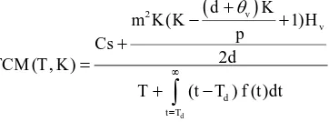
Substitute the uniform probability density function in (8), the supply chain total cost per unit time can be modeled as:

time minus production period. So the non production period can be modeled as:

(3)

C ( , K

S b θv

b

H ( θb K K ( θv K

θbK 2 θb

2 θb

θbK 2 θb Kθb KHb

⬚

2 θb

θb 2 θb

θb

KHb

b 1 d+θvP �

� Substitute (4) to (10), one has;

( θv ₍₁₁₎

Substitute (11) to (9), one has:

(12)

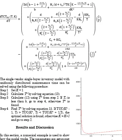
The optimal replenishment period is found by deriving (12) in term of

T

and set the value equal to 0,

one has;

C KC S b 1 d+θvP

b Hv( θb (d+θv K_P 1

( θbTK )

θ_b tbT_K

(1 θbT_K ) θ_b

Hb

( θbTK )

θ_b( θbT_K)

(1 θbT_K ) θ_b

b 1 d+θv_P � �

1

(b−1+d+θv_�P )�

= 0 (13)

If the optimal production down time is bigger than the upper bound of the uniform distribution unavailable time, then lost sales will not occur. In this situation, equation (12) is not fulfilled. Equation (12) should be revised as follow:

(4)

The single-vendor single-buyer inventory model with uniformly distributed maintenance time can be solved using the following procedure:

Step 1 Set K = 1

Step 2 Calculate T* by solving equation (13) Step 3 Calculate (12) using T* from step 2. If Td is

less than b, go to step 4, otherwise T* is found.

Step 4 Find T* by solving equation 15. If TUC(K* - 1, T) > TUC(K*, T) < TUC(K* + 1,T), the optimal solution is found, otherwise K = K+1 and go to step 2.

Results and Discussion

In this section, a numerical example is used to show how the model works. The parameters are setup cost (Cs) $40/ set up, transportation cost (Ct) $ 0.5/ delivery, production rate (p) 150 per unit time, demand rate (d) 80 per unit time, manufacture holding cost (Hv) $ 5/unit/unit time, buyer holding cost (Hb) $ 6/unit/unit time, buyer lost sales cost (S) $ 12/unit, manufacture deteriorating rate (θv)

0.05/unit time, and buyer deteriorating rate (θb)

0.06/unit time. Manufacture unavailability time is uniformly distributed between 0 and 1. Due to complexity of the model, a closed form solution can not be derived and the model is solved using simple heuristic method using Maple software. The optimal total cost can be derived when replenishment period is small but larger than zero.

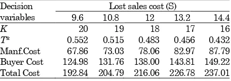
Figure 3 shows total cost in varies value of T, when K is equal to 3.

Figure 3 Total cost in varies of T

Table 1. The computational results for Uniform distri-bution unavailability time

K T* TCT* ($) K T* TCT* ($)

1 0.346 473.77 11 0.457 219.98 2 0.390 330.42 12 0.463 218.70 3 0.409 283.00 13 0.467 217.75 4 0.421 259.71 14 0.470 217.07 5 0.429 246.11 15 0.474 216.60 6 0.436 237.35 16 0.477 216.29 7 0.441 231.36 17 0.480 216.11 8 0.446 227.10 18 0.483 216.06

9 0.451 224.00 19 0.487 216.09 10 0.455 221.70 20 0.490 216.21

C NL( , K

S b θv

b

H ( tb K K ( θv K

θbK 2 θb

2 θb

θbK 2 θb Kθb KHb

2 θb

θb 2 θb

θb

KHb

(_�)

The optimal replenishment time for total cost without lost sales can be found by deriving (14) in term of T, and one has:

C KC

S b 1 d+θv_P b

Hv( θb (d+θv K_P 1

θbTK

θ_b θbT_K

1 θbT_K θ_b

Hb

θbTK

θ_b θbT_K

1 θbT_K

θ_b

b 1 d+θv_P � �

1

(5)

Table 2. Sensitivity analysis for Uniform distribution unavailability time.

Decision variables

Lost sales cost (S)

9.6 10.8 12 13.2 14.4

K 20 19 18 17 16

T* 0.552 0.515 0.483 0.456 0.432 Manf.Cost 67.86 73.03 78.06 82.97 87.79 Buyer Cost 124.98 131.76 138.00 143.81 149.22 Total Cost 192.84 204.79 216.06 226.78 237.01

Table 1 shows the computational results of the numerical example. The optimal total cost per unit time is derived when the number of delivery (K) is equal to 18. The optimal total cost per unit time is equal to $ $216.06 and the optimal production time is 0.483. Since the lost sales cost is one of the important parameters, then a sensitivity analysis is conducted in different value of lost sales cost (S). The sensitivity analysis results is shown in Table 2.

The sensitivity analysis shows that the lost sales cost significantly affect the optimal total cost. When the lost sales cost increase 20%, the optimal total supply chain cost increase 9.6%. The optimal total cost increase as the lost sales cost increase. The result is similar as many previous research. The optimal frequency of delivery and the optimal replenishment time decrease as the lost sales cost increase. Manu-facture and buyer try to minimize their cost by reducing their replenishment time and the frequency of delivery. The total cost per unit time of manufacture and buyer increase as the lost sales cost increase. Since the buyer reducing his replenishment period, the manufacture cost per unit time increase. The manufacture cost per unit time increase 12,46% and the buyer cost per unit time increase 8.13% as the lost sales cost increase 20%. Percentage increasing cost per unit time of manu-facture higher than percentage increasing cost per unit time of the buyer. However manufacture cost is less than the buyer cost. In the supply chain model, the supply chain leader gets more benefit in a supply chain. Manufacture should give compensation to the buyer to make the buyer buy more products from the manufacture and reducint manufacture cost per unit time.

Conclusion

In this paper, a deteriorating production inventory model for two echelons supply chain by considering unreliable production system is developed. Uniform distributions of machine unavailability time are considered in this research. A simple heuristic method is used to solve the model since a closed form

solution can not be derived. A numerical example and a sensitivity analysis are derived to verify the model. The sensitivity analysis shows that the total supply chain cost per unit time increase as the lost sales cost increase. Manufacture cost per unit time increase as the lost sales cost increase because the buyer tries to minimize his cost by redusing reple-nishment period. The research can be extended by considering some manufacture strategies to in-fluence buyer to buy more productsin unreliable machine environment.

Acknowledgement

The work is supported by research grant from Indonesia Ministry of Education (Number: 25/SP2H/ PP/LPPM-UKP/II/2012)

References

1. Misra, R.B., Optimum Production Lot-Size Model for a System with Deteriorating Inventory, International Journal of Production Research, 13, 1975, pp. 495-505.

2. Zequeira, R.I., Valdes, J.E., and Berenguer, C., Optimal Buffer Inventory and Opportunistic Preventive Maintenance under Random Product-ion Capacity Available, International Journal of Production Economics, 111, 2008, pp. 686-696. 3. Abboud, N.E., Jaber, M.Y., and Noueihed, N.A.,

Economic Lot Sizing with the Consideration of Random Machine Unavailability Time, Com-puters & Operations Research, 27, 2000, pp. 335 – 351.

4. Chung, C.J., Widyadana, G.A., and Wee, H.M., Economic Production Quantity Model for Deteriorating Inventory with Random Machine Unavailability, International Journal of Produc-tion Research, 49 (3), 2011, pp. 883-902.

5. Wee, H.M., and Widyadana, G.A., Economic Production Quantity Models for Deteriorating Items with Rework and Stochastic Preventive Maintenance Time, International Journal of Production Research, 50(11), 2012, pp. 2940-2952.

6. Wee, H.M., and Widyadana, G.A., Single Vendor Single Buyer Inventory Model with Discrete Delivery Order, Random Machine Unavailability and Lost Sales, International Journal of Production Economics, 143(2), 2013, pp. 574-579. 7. Rau, S., Wu, M.Y., and Wee, H.M., Integrated