EFFICIENT RECONSTRUCTION OF LARGE UNORDERED IMAGE DATASETS
FOR HIGH ACCURACY PHOTOGRAMMETRIC APPLICATIONS
Mohammed Abdel-Wahab, Konrad Wenzel, Dieter Fritsch
ifp, Institute for Photogrammetry, University of Stuttgart Geschwister-Scholl-Straße 24D, 70174 Stuttgart, Germany {mohammed.othman, konrad.wenzel, dieter.fritsch}@ifp.uni-stuttgart.de
Commission III, WG I
KEY WORDS: Photogrammetry, Orientation, Reconstruction, Incremental, Adjustment, Close Range, Matching, High Resolution
ABSTRACT:
The reconstruction of camera orientations and structure from unordered image datasets, also known as Structure and Motion reconstruction, has become an important task for Photogrammetry. Only with few and rough initial information about the lens and the camera, exterior orientations can be derived precisely and automatically using feature extraction and matching. Accurate intrinsic orientations are estimated as well using self-calibration methods. This enables the recording and processing of image datasets for applications with high accuracy requirements. However, current approaches usually yield on the processing of image collections from the Internet for landmark reconstruction. Furthermore, many Structure and Motion methods are not scalable since the complexity is increasing fast for larger numbers of images. Therefore, we present a pipeline for the precise reconstruction of orientations and structure from large unordered image datasets. The output is either directly used to perform dense reconstruction methods or as initial values for further processing in commercial Photogrammetry software.
1. INTRODUCTION
Structure and Motion(SaM) methods enable the reconstruction of orientations and geometry from imagery with little prior information about the camera. The derived orientations are commonly used within dense surface reconstruction methods which provide point clouds or meshes with high resolution. This modular pipeline is employed for different applications as an affordable and efficient approach to solve typical surveying tasks.
One example is the use of unmanned aerial vehicles (UAVs) in combination with a camera. For many tasks, such as the survey of a golf court or the survey of a construction site progress, the use of a manned aircraft in combination with classical photogrammetric methods would be ineffective and too expensive. Thus, additional market potential can be exploited by such UAV surveying in combination with automatic image processing software.
Especially for low cost application, where a small fixed wing remote controlled airplane is used in combination with a consumer camera, this approach enables the surveying of large area at low costs. As shown by [Haala et al., 11], SaM reconstruction methods can be used to derive digital surface models and orthophotos. However, the current challenge is the processing of very large number of images at a reasonable time since the complexity of the SaM methods is typically increasing nonlinear.
Another challenge is the derivation of orientations for applications with high accuracy requirements. One example is close range photogrammetry data recording for the derivation of point clouds with sub-mm precision, such as [Wenzel et al., 11]. Within this project about 2 billion points were derived using about 10,000 images and a software pipeline incorporating Structure from Motion reconstruction and dense image matching methods. Thus, a method capable of processing very large image datasets with high accuracy was required here.
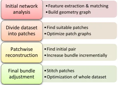
Therefore, we present a pipeline that was developed focusing on efficiency and accuracy. As shown in figure 1, it is divided into four processing steps. It employs an initial image network analysis in order to avoid the costly matching of all possible image pairs and to guide the reconstruction process. The following tie point generation is designed to derive points with maximum accuracy and reliability. By building and optimizing a geometry graph based on the image network, the dataset can be split into reliable patches of neighboring images which can be processed independently and in parallel within the reconstruction step. Finally, all these patches are merged and optimized by a global bundle adjustment. Ground control points can be integrated within this step as well.
In order to achieve a maximum accuracy a camera calibration is required. Current Structure and Motion implementations use self-calibration methods where the focal length and the radial distortion are usually determined within the bundle adjustment for each station individually. However, if the accuracy requirements of the application are high and a camera with high stability and fixed focal length is employed we use calibration parameters determined prior by standard calibration methods.
•Feature extraction & matching •Build geometry graph
Initial network analysis
•Find suitable patches •Optimize patch graphs
Divide dataset into patches
•Find initial pair
•Increase bundle incrementially
Patchwise reconstruction
•Stitch patches
•Optimization of whole dataset
Final bundle adjustment
Figure 1. Flowchart for the presented pipeline ISPRS Annals of the Photogrammetry, Remote Sensing and Spatial Information Sciences, Volume I-3, 2012
2. RELATED WORK
In the past few years, the massive collection of imagery on the Internet and ubiquitous availability of consumer grade compact cameras have inspired a wave of work on SaM— the problem of simultaneously reconstructing the sparse structure and camera orientations from multiple images of a scene. Moreover, the research interest has been shifted towards reconstruction from very large unordered and inhomogeneous image datasets. The current main challenges to be solved are scalable performance and the problem of drift due to error propagation.
Most SaM methods can be distinguished into sequential methods starting with a small reconstruction and then expanding the bundle incrementally by adding new images and 3D points like [Snavely et al., 07] and [Agarwal et al., 09] or hierarchical reconstruction methods where smaller reconstructions are successively merged like proposed by [Gherardi et al., 10]. Unfortunately, both approaches require multiple intermediate bundle adjustments and rounds of outlier removal to minimize error propagation as the reconstruction grows due to the incremental approach. This can be computationally expensive for large datasets.
Hence, recent work has used clustering [Frahm et al., 10] or graph-based techniques [Snavely et al., 2008] to reduce the number of images. These techniques make the SaM pipeline more tractable, but the optimization algorithms themselves can be costly. Furthermore, we focus on datasets where one cannot reduce the number of images significantly without losing a substantial part of the model since no redundant imagery is available.
In order to increase the efficiency of our reconstruction we employ a solution called partitioning methods like proposed by [Gibson et al., 02] and as used in [Farenzena et al., 09 & Klopschitz et al., 10]. Within this partitioning approach the reconstruction problem is reduced to smaller and better conditioned sub-groups of images which can be optimized effectively. The main advantage of this approach is that the drift within the smaller groups of images is lower which supports the initialization of the bundle adjustment. Therefore, we split up our dataset into patches of a few stable images, perform an accurate and robust reconstruction for each of it and merge all patches within a global bundle adjustment.
3. INITIAL NETWORK GEOMETRY ANALYSIS
This step is designed to accurately and quickly identify image connections for unordered collections of photos. A connectivity graph is the output of this step and is used as a heuristic about the quality of connections between the images. In addition, this connectivity graph reveals singleton images and small subsets that can be excluded from the dataset. Finally, it is used to guide the process of pairwise matching (sec. 3.2) instead of trying to match every possible image pair. In order to calculate the geometry graph, the images are matched to each other pair-wise, followed by a geometry verification step.
3.1 Similarity measures
Recent developments regarding image similarities analysis can be distinguished into two major categories according to the type of image representation [Aly et al., 10]. Local feature based approaches use quality measures of matched local descriptors. In contrast, global feature based approaches utilize matching histograms describing the full image by visual words.
In practice, it can be considered that both of these categories represent the same approach, which uses data structures to perform the fast approximate search in the feature database. It is performed with varying degrees of approximation to improve speed and storage requirements. Recent research showed that the best performance can be achieved by using local feature based approaches in combination with an approximate nearest neighbor search using a forest of kd-trees if only thousands of analogy with [Brown and Lowe, 03 & Farenzena et al., 09]. In order to improve the effectiveness of the representation in higher dimensions, all descriptors are stored using a randomized forest of kd-trees. nearest neighbors. Afterwards, the weighted number of matches between each pair is stored in a 2D histogram where all features with a distance more than a certain threshold are considered to be outliers. We use twice the standard deviation of the distances of closest neighbors as threshold value.
Connectivity graph: The inverse of the distances between matched feature pairs are used as weights for similarity. Furthermore, we introduce additional quality measures for the similarity between images such as the approximate image overlap derived from the convex hull of the matched feature points. The quality measures are normalized and summarized to one single quality value, which is stored in the index matrix. Finally, this index matrix is binarized using three thresholds to determine initial probable connections and disconnections.
3.2 Keypoint matching
Matching each connected image pair is accomplished using the connectivity matrix obtained during the previous step (sec. 3.1). Thus, corresponding 2D pixel measurements are determined between all connected image pairs. For that, we follow the approach presented in [Farenzena et al., 09]. In particular, a set of candidate features are matched using a kd-tree procedure based on the approximate nearest neighbor algorithm. This step is followed by a refinement of correspondences using an outlier rejection procedure based on the noise statistics of correct and incorrect matches. The results are then filtered by a standard RANSAC based geometric verification step, which robustly computes pairwise relations.
Homography and fundamental matrices are used with an efficient outlier rejection rule called X84 [Hampel et al., 86] to increase reliability and accuracy. Finally, the best-fit model is selected according to the Geometric Robust Information Criterion (GRIC) [Torr, 97] as initial model for the reconstruction.
Algorithm 1. Building graph for patches
Input: geometry graph
Output: collection of patches graph 1. Set new empty graph (patch) { } 2. Determine most reliable edge in
3. Add and its vertices into 4. Set in
5. in connected at least with two vertices in
If & Add into
Set in
6. Add edges in between inliers vertices in 7. set all these edges in
8. Repeat steps 4,5 and 6 until in step 4 9. Store and repeat steps 1:7 until all edges in
3.3 Geometry graph
Afterwards, a weighted undirected geometry graph, is constructed where is a set of vertices and is a set of edges. Thus, two view relations are encoded such that each vertex refers to an image while each weighted edge presents the overlap between the corresponding image pair. The weights of the edges are stored according to the number of their shared matching points and the overlap area between view images and .
4. PATCHWISE RECONSTRUCTION
In order to speed up the reconstruction of large datasets and to reduce the drift problem we follow a partitioning approach. Therefore, we divide the dataset into overlapping patches where each patch contains a manageable size of images. Thus, a parallelizable process replaces the process of reconstructing the whole scene at once where the large number of iterations with the growing number of unknowns can lead to very high computation times for complex datasets.
4.1 Dataset splitting into patches
The idea is to start multiple reconstructions beginning at image connections with high overlap in order to ensure a reliable geometry. As shown in algorithm 1, we select an initial pair according to the most reliable edge being identified by its weights within the geometry graph. The graph of this patch is then extended using the neighboring edges with highest weights until a predefined number of images or patch graph level is reached. Also, only reliable connections are identified according to thresholds on the weights of the geometry graph edges to ensure the highest mutual compatibility.
Furthermore, only images overlapping with at least two more images are considered. While the patch graph is growing, each used edge is eliminated in the geometry graph. As soon as the patch graph is finalized, the whole procedure is repeated to find the next patch until all imagery is covered. The overlap between
the final patches is ensured by considering and removing edges only instead of cameras. Thus, common cameras remain.
4.2 Keypoint tracking
Once a graph is determined for each patch as described in the previous section, we can start the optimization process as following. We track the keypoints over all images in each patch and store the results in a separated visibility matrix, which depicts the appearance of points in the images. Subsequently, a filtering is applied where all points visible in less than 3 images are eliminated. Furthermore, tracks are rejected which have measurements with converging image coordinates in common.
4.3 Dynamic keypoint filtering
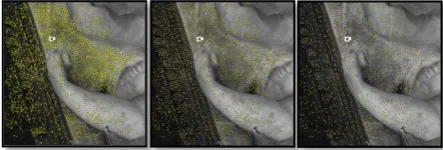
For more efficiency, we apply a homogeneous and dynamical filtering (see figure 2) approach for the tracked points to keep only the points with the highest connectivity. For each image we sort the keypoints in descending order according to their number of projections in other images. Then, the point with the greatest number of projections is visited, followed by identification and rejection of all nearest neighbor points with a distance less than a certain threshold (e.g. 20 pixels). This step is repeated until the end of the points list.
In order to maintain continuity, all points selected in an image process must be considered as filtered (fixed) in the following filtering of other images. Filtering is done before the actual reconstruction step (section 3.1) in order to increase the accuracy but also to reduce the number of obsolete observations. Consequently, the geometric distribution of keypoints is improved, which reduces computational costs significantly without losing geometric stability.
4.4 Patch graph optimization
Once correspondences have been tracked and filtered, we optimize the patch graph such that we construct a weighted undirected epipolar graph for each patch containing common tracks. The weight of an edge represents the number of common points between the corresponding image pair. Then we build the edge dual graph of , where every node in corresponds to an edge in . Two nodes in are connected by an edge if and only if the corresponding image pairs share a camera and 3D points in common. Thus, each edge represents an image pair with sufficient overlap. Note that even when is fully connected any spanning tree of may be disconnected. This can happen if a particular pairwise reconstruction did not have 3D points in common with another pair.
Figure 2. Point distribution in the image space before and after filtering (3395, 2007 and 819 points according to a
filtering distance of 0, 20 and 40 pixels) ISPRS Annals of the Photogrammetry, Remote Sensing and Spatial Information Sciences, Volume I-3, 2012
Thus, we use three images as basic geometric entity by using only points that were tracked in at least three images. These points are used to build the graph in order to guarantee full connection for any sub sequential image. The maximum spanning tree (MST), which minimizes the total edge cost of the final graph is then computed. The image relation retrieved as graph is used the guide a stable reconstruction process
with minimized computational efforts.
4.5 Reconstruction initialization
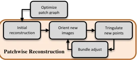
The incremental reconstruction step begins with the reconstruction of orientation and 3D points for an initial image pair as shown in figure 3. The choice of this initial pair is very important for the following reconstruction of the scene.
The initial pair reconstruction can only be robustly estimated if the image pair has at the same time a reasonable large baseline for high geometric stability and a high number of common feature points. Furthermore, the matching feature points should be distributed well in the images in order to reconstruct a maximum of initial 3D structure of the scene and to be able to determine a strong relative orientation between the images.
Find the initial pair: The most suitable initial image pair has to meet two conditions: the number of matching points must be acceptable and the fundamental matrix must explain that the matching points are far better than homography models. For that, GRIC scores are employed as used in [Farenzena et al., 09].
Reconstruct initial pair: The extrinsic orientation values are determined for this initial pair by factorizing the essential matrix and the tracks visible in the two images. A two-frame bundle adjustment starting from this initialization is performed to improve the reconstruction.
Add new images and points: After reconstructing the initial pair additional images are added incrementally to the bundle. The most suitable image to be added is selected according to the maximum number of tracks from 3D points already being reconstructed. Within this step not only this image is added but also neighboring images that have a sufficient number of tracks as proposed by [Snavely et al., 07]. Adding multiple images at once reduces the number of required bundle adjustments and thus improves efficiency.
Next, the points observed by the new images are added to the optimization. A point is added if it is observed by at least 3 images, and if the triangulation gives a well-conditioned estimate of its location. This procedure follows the approach of [Snavely et al., 07] as well. The Jacobian matrix is used during the optimization step in order to provide a computation with reduced time and memory requirements.
Sparse bundle adjustment after each initialization: once the new points have been added, a bundle adjustment is performed on the entire model. This procedure of initializing a camera orientation, triangulating points, and running bundle adjustment is repeated, until no images observing a reasonable number of points remain. For the optimization we employ the sparse
bundle adjustment implementation “SBA” [Lourakis, A., & Argyros, A., 09]. SBA is a non-linear optimization package that takes advantage of the special sparse structure of the Jacobian matrix used during the optimization step in order to provide a computation with reduced time and memory requirements.
5. GLOBAL BUNDLE ADJUSTMENT
After the reconstruction of points and orientations for the overlapping patches the results are merged. Since outlier rejection was performed within the previous processing the available 3D feature points are considered to be reliable and accurate. Due to the overlap the patches have a certain number of points and camera orientations in common which enable the determination of a seven-parameter transformation to align the patches into a common coordinate system. The transformed orientations and points are introduced into a common global bundle adjustment of the whole block. If ground control point measurements are available they can be used for the improvement of the bundle and to enable georeferencing.
6. RESULTS
The derived orientation and sparse point cloud can be used for further processing to derive photogrammetric products like dense point clouds or orthophotos. Therefore, we employ a dense image matching pipeline using a hierarchical multi-stereo method to derive dense point clouds while being scalable for large datasets [Wenzel et. al., 11]. Another option is to use the output of the pipeline in commercial Photogrammetry software such as Trimble Match-AT to refine the bundle adjustment or to derive surface models and orthophotos.
6.1 Close range photogrammetry
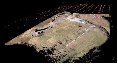
Within a cultural heritage recording project 10,000 images were recorded using a multi camera rig at short acquisition distance [Fritsch et al., 11 and Wenzel et al., 11]. The exterior orientations for the images were derived without initial values using the presented pipeline with high accuracy requirements. By performing a dense image matching step 2 billion points Patchwise Reconstruction
Initial reconstruction
Orient new images
Tringulate new points
Bundle adjust Optimize
patch graph
Figure 3. Flowchart for the patchwise reconstruction
Figure 4. Camera stations (red), sparse point cloud from the SaM reconstruction (right) and point cloud derived by dense image matching (left) for a cultural heritage recording dataset ISPRS Annals of the Photogrammetry, Remote Sensing and Spatial Information Sciences, Volume I-3, 2012
could be derived with sub-mm resolution (extract shown in figure 4). The high requirements of the orientations were met, as evaluated in section 7.
6.2 Unmanned Aerial Vehicles (UAV)
The increasing use of unmanned aerial vehicles for surveying tasks such as construction site progress documentation or surface model generation of small areas requires a method to derive spatial data at low costs. Typically, UAVs are equipped with consumer cameras providing a small footprint only. The imagery is challenging since the signal to noise ratio is low due to the small pixel pitch.
Furthermore, the movements of the small aircraft in case of a fixed wing lead to a significant image blur as also present for the datasets presented in [Haala et al., 11]. Within this investigation the presented pipeline was applied to derive orientations and tie points (figure 5). The small footprint of the consumer camera led to dataset of 1204 images, where about 230 images were eliminated before the processing because of image blur or low connection quality. From the remaining 975 images 959 could be oriented successfully. Even though an image blur of up to a few pixels was present for most images the bundle adjustment succeeded with a mean reprojection error of 1.1 pixels.
7. EVALUATION
7.1 Relative accuracy
In order to assess the relative accuracy of the results derived by the presented Structure and Motion reconstruction pipeline we analyzed control point measurements in the close range cultural heritage data recording project. About 100 targets are distributed over the whole object and are used in a later step for georeferencing. The control points are captured in 12 independent datasets, represented by the 6 individually processed patches for the two facades.
The shape of each target is a black circle with 20mm diameter and a white inner circle with 5mm diameter. The white circle is detected and measured in the image automatically using an ellipse fit. These image measurements are considered to have an accuracy of about 0.1pixels.
Until this point the control points are not used in the bundle and thus do not impact the orientations to be evaluated. Consequently, they can be used to assess the quality using the triangulation error represented by the discrepancy of the rays to be intersected. Since all orientations are in a local coordinate system and since the intersection geometry differs, the projected error in image space is evaluated instead of the error in object
space. Within the evaluation strategy the targets are identified and measured in the images. For each control point the corresponding image measurements are used together with the relative orientation to triangulate an object coordinate.
About 6 projections per control point were averagely used for the triangulation. If the reprojection of a measurement exceeds a threshold of 1pixel it is considered to be a false measurement and eliminated.
As shown in figure 6 and table 1, the root mean square of the reprojection error for each dataset is about 0.3 pixels. At 70cm distance this corresponds to an error of approximately 0.2mm for the image scale of this dataset. This is considered to meet the requirements for the later dense surface reconstruction step, where a relative accuracy in image space of better than 0.5 pixels is required for a reliable image matching.
7.2 Absolute accuracy
After the automatic measurement and triangulation of control points, coordinates in object space are available for each control point. These coordinates in the local coordinate system defined during the Structure and Motion reconstruction can be used for georeferencing. Therefore, the control points were measured by reflectorless tachymetry.
The mean standard deviation determined by the network adjustment amounts to 1.4mm in position and 1.6mm in height. However, many points were occluded and thus could not or only once be measured. Consequently, no accuracy information could be determined for these values. The residuals after the estimation of a rigid seven-parameter transformation in millimeters are presented in Table 2. The mean RMS for the 12
Data Points Proj. Min Max Mean RMS
Set 01 20 163 0,016 0,998 0,305 0,388
Set 02 12 063 0,009 0,556 0,141 0,185
Set 03 11 052 0,008 0,552 0,212 0,267
Set 04 13 080 0,014 0,793 0,213 0,266
Set 05 05 017 0,042 0,787 0,286 0,360
Set 06 09 055 0,017 0,640 0,159 0,212
Set 07 24 176 0,005 0,828 0,194 0,258
Set 08 11 065 0,003 0,875 0,199 0,262
Set 09 12 085 0,010 0,943 0,199 0,263
Set 10 15 097 0,013 0,929 0,237 0,308
Set 11 13 095 0,028 0,859 0,199 0,256
Set 12 15 114 0,002 0,909 0,197 0,265
Mean 13,3 88,5 0,014 0,806 0,212 0,274
Table 1. Reprojection error in pixels for 1062 target measurements in 12 independent datasets. The targets were
automatically measured and subsequently triangulated. Columns: point count, number of projections, minimum
reprojection error, maximum, mean and RMS. Figure 5. Sparse point cloud and camera stations (red) for an
image dataset acquired by an UAV
Figure 2. Histogram of the reprojection error for all measurements of all datasets.
0 0.1 0.2 0.3 0.4 0.5 0.6 0.7 0.8 0.9 1
0 20 40 60
Reprojection error [pixel] ISPRS Annals of the Photogrammetry, Remote Sensing and Spatial Information Sciences, Volume I-3, 2012
datasets is 2.2mm. The number of used control points is less than in the previous analysis, since reference measurements from tachymetry are not available for all points.
However, the RMS values derived from the residuals after the seven-parameters cannot be used for an absolute accuracy assessment, since a reference measurement with the accuracy of one magnitude higher would be required. In contrast, the accuracy of the tachymetric measurements is in a similar range. Thus, these values are only used to validate the reconstructed orientations in object space.
8. CONCLUSION
The presented pipeline is capable of reconstructing orientations and sparse point clouds with high accuracy. Splitting up the dataset into suitable sub-groups of images not only enables scalability due to a faster and parallelizable reconstruction process. Also, the drift is reduced implicitly since the reconstruction starts at the most reliable parts and thus minimizes the propagation of errors. Thus, precise orientations can be derived for large and complex datasets. Within further processing the derived orientations can be used for dense surface reconstruction methods or other further processing with other Photogrammetry software.
1. REFERENCES
Agarwal, S., Snavely, N., Simon, I., Seitz, S., Szeliski, R., 2009. Building Rome in a Day, ICCV, 2009.
Aly, M., Munich, M., and Perona, P., 2011. Indexing in Large Scale Image Collections: Scaling Properties and Benchmark, 2011. IEEE Workshop on Applications of Computer Vision (WACV).
Bay, H., Ess, A., Tuytelaars, T., Luc, V., G., 2008. SURF: Speeded Up Robust Features, Computer Vision and Image Understanding (CVIU), pp. 346-359.
Brown, M. and Lowe, D., 2003. Recognizing panoramas. In Proc. of the 9th ICCV, Vol. 2, pp. 1218–1225.
Farenzena, M., Fusiello, A. and Gherardi, R., 2009. Structure and motion pipeline on a hierarchical cluster tree. ICCV
Workshop on 3-D Digital Imaging and Modeling, pp. 1489– 1496.
Frahm, J., Fite-Georgel, P., Dunn, E., Hill, C., 2011. State oft he Art and Challenges in Crowd Sourced Modeling. Photogrammetric Week 2011, Wichmann Verlag, Berlin/Offenbach, pp. 259-266.
Fritsch, D., Khosravani, A. M., Cefalu, A. and Wenzel, K., 2011. Multi-Sensors and Multiray Reconstruction for Digital Preservation, Photogrammetric Week 2011, Wichmann Verlag, Berlin/Offenbach, pp. 305-323.
Gherardi, R., Farenzena, M., Fusiello, A., 2010. Improving the efficiency of hierarchical structure-and-motion. In: CVPR. (2010).
Gibson, S., Cook, J., Howard, T., Hubbold, R. and Oram, D., 2002. Accurate Camera Calibration for Off-Line, Video-Based
Augmented Reality. IEEE and ACM Int’l Symp. Mixed and
Augmented Reality, pp. 37-46.
Haala, N., Cramer, M., Weimer, F. and Trittler, M., 2011. Performance Test on UAV-based data collection. Proc. of the International Conf. on UAV in Geomatics. IAPRS, Volume XXXVIII-1/C22, 2011.
Hampel, F., Rousseeuw, P., Ronchetti, E. and Stahel, W., 1986. Robust Statistics: The Approach Based on Influence Functions, ser. Wiley Series in probability and mathematical statistics. New York: Wiley, 1986.
Klopschitz, M., Irschara, A., Reitmayr, G., and Schmalstieg, D., 2010. Robust incremental structure from motion. Proc. 3DPVT.
Lourakis, A., and Argyros, A., 2009. Sba: A software package for generic sparse bundle adjustment. ACM TOMS, 36(1):pp. 1–30.
Lowe, D., 2004. Distinctive Image Features from Scale-Invariant Keypoints. International Journal of Computer Vision, Vol. 60, pp. 91-110
Muja, M. and Lowe, D., 2009. Fast approximate nearest neighbors with automatic algorithmic configuration. Proc. VISAPP.
Snavely, N., Steven M. Seitz, Richard Szeliski.Skeletal Sets for Efficient Structure from Motion. Proc. Computer Vision and Pattern Recognition (CVPR), 2008.
Snavely, N., Seitz, S. and Szeliski, R., 2007. Modeling the world from internet photo collections. International Journal of Computer Vision.
Schwartz, C., Klein, R., 2009. Improving initial estimations for structure from motion methods. In Proc. CESCG, April 2009.
Torr, P., 1997. An assessment of information criteria for motion model selection. in Proc. IEEE Conf. Computer Vision Pattern Recognition , pp. 47–52.
Vedaldi, A., and Fulkerson, B., 2008. VLFeat: An open and portable library of computer vision algorithms.
Wenzel, K., Abdel-Wahab, M., Fritsch D., 2011. A Multi-Camera System for Efficient Point Cloud Recording in Close Range Applications. LC3D workshop, Berlin, December 2011.
Data Points Min Max Mean RMS
Set 01 18 0,71 5,70 2,34 2,63
Set 02 06 0,99 2,78 2,06 2,16
Set 03 11 1,26 3,39 2,11 2,18
Set 04 13 0,59 6,33 2,79 3,25
Set 05 05 0,83 5,12 2,62 2,97
Set 06 09 1,24 5,57 2,86 3,21
Set 07 20 0,59 3,53 2,08 2,24
Set 08 09 0,69 2,79 1,41 1,59
Set 09 07 0,29 2,01 1,23 1,36
Set 10 14 0,93 4,02 1,89 2,06
Set 11 12 0,19 2,26 0,96 1,13
Set 12 15 0,45 3,34 1,66 1,90
Mean 11,6 0,73 3,90 2,00 2,22
Table 2. Control point residuals in millimeters after the estimation of a seven-parameter transformation using control points measured by tachymetry. Columns: point count, minimum reprojection error, maximum, mean, RMS