Full Terms & Conditions of access and use can be found at
http://www.tandfonline.com/action/journalInformation?journalCode=ubes20
Download by: [Universitas Maritim Raja Ali Haji], [UNIVERSITAS MARITIM RAJA ALI HAJI
TANJUNGPINANG, KEPULAUAN RIAU] Date: 11 January 2016, At: 21:01
Journal of Business & Economic Statistics
ISSN: 0735-0015 (Print) 1537-2707 (Online) Journal homepage: http://www.tandfonline.com/loi/ubes20
Varying Naïve Bayes Models With Applications to
Classification of Chinese Text Documents
Guoyu Guan, Jianhua Guo & Hansheng Wang
To cite this article: Guoyu Guan, Jianhua Guo & Hansheng Wang (2014) Varying Naïve Bayes Models With Applications to Classification of Chinese Text Documents, Journal of Business & Economic Statistics, 32:3, 445-456, DOI: 10.1080/07350015.2014.903086
To link to this article: http://dx.doi.org/10.1080/07350015.2014.903086
Accepted author version posted online: 17 Mar 2014.
Submit your article to this journal
Article views: 172
View related articles
Varying Na¨ıve Bayes Models With Applications
to Classification of Chinese Text Documents
Guoyu G
UANand Jianhua G
UOKey Laboratory for Applied Statistics of the Ministry of Education, and School of Mathematics and Statistics, Northeast Normal University, Changchun 130024, P. R. China ([email protected]; [email protected])
Hansheng W
ANGDepartment of Business Statistics and Econometrics, Guanghua School of Management, Peking University, Beijing 100871, P. R. China ([email protected])
Document classification is an area of great importance for which many classification methods have been developed. However, most of these methods cannot generate time-dependent classification rules. Thus, they are not the best choices for problems with time-varying structures. To address this problem, we propose a varying na¨ıve Bayes model, which is a natural extension of the na¨ıve Bayes model that allows for time-dependent classification rule. The method of kernel smoothing is developed for parameter estimation and a BIC-type criterion is invented for feature selection. Asymptotic theory is developed and numerical studies are conducted. Finally, the proposed method is demonstrated on a real dataset, which was generated by the Mayor Public Hotline of Changchun, the capital city of Jilin Province in Northeast China.
KEY WORDS: BIC; Chinese document classification; Screening consistency; Time-dependent classifi-cation rule.
1. INTRODUCTION
Document classification (Manevitz and Yousef2001) is an important area of statistical applications, for which many meth-ods have been developed. These methmeth-ods include linear discrim-inant analysis (Johnson and Wichern2003; Fan and Fan2008; Leng2008; Qiao et al.2010; Shao et al.2011; Mai, Zou, and Yuan2012, LDA), support vector machines (Wang, Zhu, and Zou2006; Zhang2006; Wu and Liu2007; Liu, Zhang, and Wu
2011, SVM), classification and regression trees (Breiman et al.
1998; Hastie, Tibshirani, and Friedman2001, CART),k-nearest neighbor (Ripley1996; Hastie, Tibshirani, and Friedman2001, KNN), boosting (Buhlmann and Yu2003; Zou, Zhu, and Hastie
2008; Zhu et al.2009), random forests (Breiman2001; Biau, Devroye, and Lugosi2008, RF), and many others. Recently, Wu and Liu (2013) proposed a novel SVM method for func-tional data; see also Ramsay and Silverman (2005) for more relevant discussions. However, how to construct a classification rule for usual (nonfunctional) data with a time-varying structure remains unclear. Thus, practical applications with time-varying data structures demand novel classification methods with time-dependent structures.
We propose a novel solution to address this problem called the varying na¨ıve Bayes (VNB) model, which is a natural ex-tension of the original na¨ıve Bayes model (Lewis1998; Murphy
2012, NB). The key difference is that the parameters in VNB are assumed to vary smoothly according to a continuous index vari-able (e.g., time). This generates a time-dependent classification rule. The proposed method is motivated by real applications. For example, the Mayor Public Hotline (MPH) is an important project led by the local government of Changchun city, the cap-ital city of Jilin Province in Northeast China, which has an area of 20,604 km2and a population of 7.9 million. The MPH project
gives local residents the opportunity to call the Mayor’s office and report various public issues via the appeal hotline “12345.” The typical issues reported include: local crime, education, pub-lic utility, transportation, and many others. Each phone call is recorded and converted into a text message in Chinese by an op-erator. Next, experienced staff in the Mayor’s office are required to manually classify these documents into different classes ac-cording to their corresponding functional departments in the local government (e.g., transportation department and police department).
Clearly, manually classifying these documents accurately to the correct functional departments is a challenging task, both technically and physically. Technically, there are many depart-ments in the local government. Thus, the staff responsible for this task need to be highly familiar with the structure of the entire government and the functionality of each department. Physically, the total amount of text documents that need to be processed every day is tremendous. Because the MPH project was operated successfully in previous years, the daily amount of MPH calls has increased from about 10 calls in 2000 to sev-eral thousand at present. Classifying this huge amount of docu-ments by human labor is a virtually impossible task. However, addressing this challenging task by statistical learning is a major problem.
To address this problem, we employ the concept of vector space modeling (Lee, Chuang, and Seamons1997) and collect a bag of the most frequently used Chinese keywords. These
© 2014American Statistical Association Journal of Business & Economic Statistics
July 2014, Vol. 32, No. 3 DOI:10.1080/07350015.2014.903086
445
keywords are indexed by jwith 1≤j ≤p. Subsequently, for a given document i (1≤i≤n), we define a binary feature Xij =1 if thejth keyword appears in theith document, and we defineXij =0 otherwise. In this manner, the original text docu-mentiis converted into a binary vectorXi =(Xi1, . . . , Xip)∈
{0,1}p. Because the total number of keywords (i.e.,p) involved in the MPH project is huge, the feature dimensionp is ultra-high. LetYibe the corresponding class label (i.e., the associated functional department). To solve the problem, a classification method is required so that a regression relationship can be con-structed fromXi toYi. Among the possible solutions, we find that na¨ıve Bayes (NB) is particularly attractive for the following reasons.
First, NB is theoretically elegant. More specifically, NB as-sumes that different binary features are mutually independent after conditioning on the class label. Therefore, the likelihood function can be derived analytically and the maximum likeli-hood estimator can be obtained easily. As a result, NB is com-putationally easier than more sophisticated methods, such as latent Dirichlet allocation method (Blei, Ng, and Jordan2003). In addition, the actual performance of NB on real datasets is competitive. Depending on the datasets, NB might not be the single best classification method. However, its performance is competitive across many different datasets. Thus, it has been ranked as one of the top ten algorithms in data mining; see, for example, Lewis (1998) and Wu and Kumar (2008). It is remark-able that some other popular document representation schemes, such as term (keyword) frequency-inverse document frequency (Salton and McGill 1983), do not perform well on the MPH dataset. This is because the frequencies of most keywords are extremely low in a single document. They are either one or zero in most cases, because the majority of keywords appear no more than once in each document.
Despite its popularity in practice, the performance of NB can be improved further. This is particularly true for the MPH dataset. In particular, we find that MPH documents recorded at different times of day (i.e., the recording time) might fol-low different classification patterns. For example, traffic is-sues are more likely to be reported during rush hour and less likely at midnight. Unfortunately, the classical NB method cannot use this valuable information. As a result, its predic-tion accuracy is suboptimal. This motivated us to develop the VNB method. This new method adopts a standard na¨ıve Bayes formulation for documents recorded at the same time of day. However, the documents recorded at different record-ing times are allowed to have different classification patterns. This is achieved by allowing the model parameters to vary smoothly and nonparametrically according to the recording time. Kernel smoothing technique is used to estimate the un-known parameters, and a BIC-type criterion is proposed to iden-tify important features. The new method’s outstanding perfor-mance is confirmed numerically on both simulated data and the MPH datasets. Our research is motivated by the MPH project, but the methodology we have developed is applicable to any classification problems with binary features and time-varying structures.
The remainder of this article is organized as follows. The next section describes the VNB method. The methods used for
parameter estimation and feature screening (Fan and Lv2008; Wang 2009) are also discussed. Numerical studies based on both simulated data and the MPH datasets are presented in Section3. Finally, the article concludes with a brief discussion in Section 4. All of the technical details are provided in the Appendix.
2. THE METHODOLOGY DEVELOPMENT
2.1 Varying Na¨ıve Bayes Model
Recall that each MPH record is indexed byiwith 1≤i≤n. The associated high-dimensional binary feature is given by Xi =(Xi1, . . . , Xip)∈ {0,1}p, and the corresponding class la-bel is recorded byYi ∈ {1, . . . , m}. DefineP(Yi =k)=πkand P(Xij =1|Yi =k)=θkj. Then, a standard na¨ıve Bayes (NB) model assumes that
P(Xi =x|Yi=k)= p
j=1
θxj
kj(1−θkj)1−xj,
wherex =(x1, . . . , xp) ∈ {0,1}prepresents a particular real-ization ofXi. Next, we useUito denote the index variable (i.e., the recording time) of theith document. Without loss of gen-erality, we assume thatUi has been standardized appropriately such thatUi ∈[0,1]. To takeUiinto consideration, we propose the following varying na¨ıve Bayes (VNB) model,
P(Xi =x|Yi =k, Ui =u)= p
j=1
{θkj(u)}xj{1−θkj(u)}1−xj,
(2.1)
where u is a particular realization of Ui, θkj(u)=P(Xij = 1|Yi =k, Ui =u), andP(Yi =k|Ui =u)=πk(u). Bothθkj(u) andπk(u) are assumed to be unknown but smooth functions inu. In other words, we assume that different features (i.e.,Xij) are independent, conditional on the class label (i.e.,Yi), and index variable (i.e.,Ui).
Clearly, the key difference between NB and VNB is that VNB allows the model parameters (i.e.,θkjandπk) to be related non-parametrically to the recording timeu. As a result, VNB adopts a standard NB formulation for documents recorded at the same time of day. However, the classification patterns of documents with different recording times are allowed to be (but not nec-essarily) different. In an extreme situation, if the classification pattern does not change according to the recording time, the parameters involved in (2.1) become constants. Thus, the VNB model reduces back to a standard NB model. Therefore, VNB contains NB as a special case. However, if the classification pattern does change according to the recording time, VNB has a much greater modeling capability and classification accuracy. To estimate the unknown parameters, we employ the concept of local kernel smoothing (Fan and Gijbels1996), which yields
the following simple estimators, functionK(t) is a probability density function symmetric about 0. Then, based on (for example) the results of Li and Racine (2006), we know that these two estimators are consistent, as long ash→0 andnh→ ∞. Following Li and Racine (2006), we seth=αn−1/5, whereαis a tuning constant that needs to be selected based on the data. In practice, different α values should be used in the numerators and denominators of (2.2) and (2.3), for differentkandj. These are selected by minimizing the cross-validated misclassification error. To simplify the notation, we use a commonαthroughout the rest of this study. Thus, the posterior probability can be estimated as
Subsequently, the unknown functional department of a new observation with X0 =x and U0 =u can be predicted as
ˆ
Y0=argmaxkP(Y0=k|X0=x, U0=u).
2.2 Feature Selection
Because the total number of frequently used Chinese key-words is huge in the MPH project, the feature dimensionpis ultrahigh. However, most of the keywords (or features) are irrel-evant for classification. As a result, the task of feature screening (Fan and Lv2008; Wang2009) becomes important. Intuitively, if a featurejis irrelevant for classification, its response proba-bility, that is,θkj(u), should be the same across all the functional departments (i.e.,k) and for almost all of the recording time (i.e., u). Thus, we haveE{θkj(Ui)−θj(Ui)}2=0 for everyk, where
θj(u)=P(Xij =1|Ui =u)=kπk(u)θkj(u). By contrast, if a featurejis relevant for classification, the response probability θkj(u) will be different for at least two functional departments and for a nontrivial amount of the recording time. As a result, we haveE{θkj(Ui)−θj(Ui)}2=0 for somek. This suggests that whether a featurej is relevant for classification is determined fully by evant for classification if and only if φj =0. Then, the true model can be defined asMT = {1≤j ≤p:φj >0}. We de-fine MF = {1, . . . , p} as the full model. We also define a generic notationM= {j1, . . . , jd}as an arbitrary model with Xij1, . . . , Xijdas relevant features. Next, for a finite dataset, the
parameterφj can be estimated as
ˆ itively, features with larger ˆφj values are more likely to be relevant for classification. By contrast, those with smaller ˆφj values are less likely to be relevant. This suggests that the true modelMT can be estimated byMc= {1≤j ≤p: ˆφj > c}, for some appropriately determined critical valuec≥0. Indeed, by the following theorem, we know thatMc is consistent for
MT, provided the critical valuecis selected appropriately.
Theorem 1. Assuming the conditions (C1)–(C4) in Appendix A, for any constant α >0 and c=2−1minj∈MTφj, we have
P(Mc=MT)→1 asn→ ∞.
2.3. Critical Value Selection
According to Theorem 1, we know thatMc is a consistent estimator ofMT, provided the critical valuecis selected appro-priately. However, the selection ofcis not clear in practice. By considering all the possiblecvalues on [0,∞), a sequence of candidate models can be generated, which constitute a solution pathM= {Mc:c≥0}. Although there are infinitely many dif-ferent choices forc, the resulting choices forMcare finite. More specifically, let{(1),(2), . . . ,(p)}be a particular permutation of
{1,2, . . . , p}such that ˆφ(1) >φˆ(2)>· · ·>φˆ(p). Thus, the solu-tion path can also be given byM= {M(d) : 0≤d ≤p}with
M(0)= ∅andM(d)= {(1),(2), . . . ,(d)}for 1≤d ≤p, which is a finite set with a total ofp+1 nested candidate models. Ac-cording to Theorem 1, we must haveMT ∈Mwith probability tending to one. Thus, the original problem of critical value de-termination forcis converted into a problem of model selection with respect toM. Then, we follow Wang and Xia (2009) and consider the following BIC-type criterion,
BIC(M)= −2n−2
where the estimated conditional probability function
of this method can be established by the following theorem in the sense of Fan and Lv (2008) and Wang (2009). Our extensive
simulation experience also suggests that this BIC-type method works quite well.
Theorem 2. Assuming the conditions (C1)–(C4) in Appendix A, for any constant α >0, we have PMT ⊂M
→1 as n→ ∞.
3. NUMERICAL STUDIES
To demonstrate the finite sample performance of the proposed VNB method, a number of simulation experiments are con-ducted and the MPH dataset is analyzed. As mentioned in Sec-tion2.1, differentαvalues should be used in the numerators and denominators of (2.2) and (2.3), for differentkandj. However, this is not feasible for ultrahigh dimensional feature because there are so many parameters. In practice, we seth=αn−k1/5in
iKh(Ui−u)Zik, andh=αn−
1/5
kj in
iKh(Ui−u)XijZik, wherenk=iZikandnkj =iZikXijare the effective sam-ple sizes of these estimators. Throughout the rest of this study, we use the Gaussian kernelK(t)=(√2π)−1exp{−t2/2}and the optimal proportionality constantαof the bandwidths is se-lected using a five-fold cross-validation by minimizing the mis-classification error. Various sample sizes, feature dimensions, and true model sizes are considered in the simulation studies. For each fixed parameter setting, 100 simulation replications are conducted. For each simulated dataset, the BIC estimator
M is obtained. The percentage of incorrect zeros (Fan and Li2001), that is, PIZ=100%× {|(MF\M)∩MT|}|MT|−1, is computed and averaged. Similarly, the percentage of cor-rect zeros is calculated, that is, PCZ=100%× {|(MF\M)∩ (MF\MT)|}{|(MF\MT)|}−1. Finally, to evaluate the classi-fication accuracy of the resulting model, another 1000 inde-pendent test samples are generated. TheM-based VNB clas-sification accuracy is then evaluated on the test samples. The
average misclassification error (AME) is computed. For compar-ison’s sake, the AME values of KNN, AdaB (Adaptive Boost-ing), RF, SVM, NB, VNBπ, and VNB but based on the true modelMT are also included. In this case, the VNBπ method refers to the classification rule (2.4) where ˆθkj(u) is replaced with ˆθkj =(iZikXij)/(
iZik). In other words, the parame-terπk(u) is still allowed to vary according tou, butθkj is fixed as a constant.
3.1 Example 1: A Na¨ıve Bayes Model
First, we consider a standard NB model, where the parameters are fixed constants that do not change according tou. Thus, the standard NB method is expected to have the best performance. By contrast, because of the unnecessary noise introduced by the recording time, the VNB method should perform worse. We then use this example to numerically investigate the efficiency loss experienced by the VNB method when the true model is actually NB.
More specifically, the recording timeUi is generated from a uniform distribution on [0,1]. Next, we generate the associated functional departmentYi ∈ {1, . . . , m}with probabilityP(Yi = k|Ui =u)=P(Yi =k)=1/mand m=3. Given Yi andUi, thejth keyword indicator Xij is generated from a binary dis-tribution with probabilityP(Xij =1|Yi =k, Ui=u)=θkjfor j ∈MT, and P(Xij =1|Yi =k, Ui =u)=θj for j /∈MT, where MT = {1, . . . , d0} is the true model with size d0. In addition,{θkj}1≤k≤m,j∈MT and{θj}j /∈MT are simulated from a
uniform distribution on [0.1,0.9]. Thus, both the parameters πk(u) andθkj(u) are actually constants that do not change ac-cording to the reac-cording timeu.
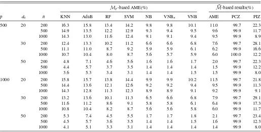
The detailed simulation results are provided inTable 1, which shows that theMT-based NB method performs best in terms of AME. This is expected because the true model is indeed NB
Table 1. Simulation results for Example 1
MT-based AME(%) M-based results(%)
p d0 n KNN AdaB RF SVM NB VNBπ VNB AME PCZ PIZ
500 20 200 16.3 15.8 13.4 14.2 9.8 9.8 10.1 11.0 99.7 22.3
500 14.9 13.5 12.2 12.9 9.3 9.4 9.5 9.6 99.9 11.7
1000 14.3 13.0 11.6 12.4 9.1 9.1 9.4 9.5 99.9 8.9
30 200 12.4 13.3 10.2 11.2 6.6 6.6 6.8 7.6 99.7 28.1
500 11.1 11.0 8.7 9.2 5.9 5.9 6.1 6.2 99.9 16.6
1000 10.7 10.4 8.0 8.7 5.6 5.7 5.9 6.0 100.0 12.2
50 200 4.8 7.1 4.6 5.6 1.6 1.6 1.7 2.0 99.7 22.3
500 4.4 5.7 3.7 3.5 1.4 1.4 1.4 1.5 99.9 12.2
1000 3.6 5.3 3.4 3.1 1.4 1.4 1.5 1.5 99.9 8.0
1000 20 200 15.8 15.7 13.8 14.4 9.9 9.9 10.2 11.5 99.7 21.8
500 14.4 13.6 12.1 12.6 9.2 9.2 9.4 9.5 99.9 11.3
1000 14.3 12.8 11.3 12.3 8.9 8.9 9.1 9.2 99.9 9.1
30 200 13.2 13.6 10.1 11.3 6.5 6.6 6.8 7.9 99.7 29.1
500 11.6 11.2 8.6 9.1 5.8 5.8 6.1 6.4 99.9 17.3
1000 10.8 10.4 8.2 8.7 5.6 5.6 5.8 6.0 99.9 11.7
50 200 5.3 7.4 4.5 5.5 1.7 1.7 1.8 2.1 99.7 23.4
500 4.5 5.7 3.6 3.5 1.4 1.4 1.5 1.6 99.9 12.3
1000 4.1 5.1 3.3 3.1 1.4 1.4 1.4 1.4 99.9 8.0
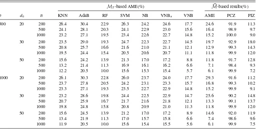
Table 2. Simulation results for Example 2
MT-based AME(%) M-based results(%)
p d0 n KNN AdaB RF SVM NB VNBπ VNB AME PCZ PIZ
500 20 200 26.4 30.4 22.9 26.3 24.2 24.6 17.7 24.6 91.9 11.3
500 24.1 28.1 20.3 24.1 22.9 23.0 15.6 16.4 98.9 9.7
1000 23.2 27.1 19.5 23.4 22.6 22.7 14.8 15.2 100.0 9.0
30 200 23.5 29.0 19.3 24.7 22.3 22.7 14.5 19.7 92.9 18.0
500 20.8 25.7 16.6 21.6 21.0 21.1 12.1 12.9 99.3 14.3
1000 19.5 24.4 15.4 20.5 20.6 20.7 11.1 11.8 99.9 12.0
50 200 15.6 24.2 13.9 21.3 17.0 17.2 8.8 11.8 91.7 12.8
500 13.2 21.4 11.3 16.9 16.1 16.2 6.6 7.1 98.4 9.3
1000 12.2 20.5 10.0 15.6 15.3 15.4 5.7 6.1 99.9 7.2
1000 20 200 26.1 30.3 22.8 26.0 23.7 24.0 17.7 29.3 91.6 11.2
500 23.7 27.8 20.5 24.2 23.1 23.3 15.7 16.8 99.3 10.2
1000 23.3 27.1 19.3 23.5 22.7 22.9 14.8 15.2 99.9 9.1
30 200 23.2 28.6 19.8 24.4 22.5 22.9 14.7 25.6 90.2 14.8
500 20.7 25.9 16.7 21.7 21.6 21.8 12.1 13.3 99.1 13.7
1000 19.8 24.8 15.8 20.8 20.9 21.0 11.3 11.8 99.9 12.0
50 200 15.6 24.5 13.9 21.2 17.0 17.2 8.9 14.6 92.0 11.9
500 13.4 21.9 11.3 17.0 15.7 15.8 6.6 7.4 98.6 9.6
1000 11.9 20.5 10.0 15.6 15.4 15.5 5.6 6.1 99.9 7.5
(not VNB). However, the performance ofMT-based VNB is comparable. This suggests that even if the true model is NB, the efficiency loss experienced by VNB is very limited. Next, we interpret the results obtained with theM-based VNB method. We find that larger sample sizenresults in smaller AME val-ues, if bothpandd0 are fixed. This is expected because larger sample size yields more accurate estimators. Furthermore, we find that the PCZ value approaches 100% and the PIZ value approaches 0% rapidly as nincreases. This confirms that the proposed BIC-type criterion is consistent for feature screening. In the meanwhile, with a fixedpandn, we find that larger true model sized0produces smaller AME values, because the inclu-sion of more relevant features improves the prediction. Finally, with a fixedd0 andn, we find that larger feature dimensionp results in worse performance in terms of AME. This is also rea-sonable because larger feature dimension is more challenging for feature screening and it results in worse prediction.
3.2 Example 2: A Varying Na¨ıve Bayes Model
We then consider a situation where the data are generated from a genuine VNB model. We aim to investigate the level of improvement obtained using VNB compared with NB and other possible competitors. More specifically, the functional depart-mentYi and the recording time Ui are generated in the same manner as Example 1 withm=3. Conditional onYi andUi, the high-dimensional featureXi is generated according to the VNB model (2.1) with
P(Xij =1|Yi=k, Ui=u)=θkj(u)
=
0.5+0.4 sin{π(u+Rkj)}, j ∈MT, 0.5+0.4 sin{π(u+R0j)}, j /∈MT,
where {Rkj}1≤k≤m,j∈MT and{R0j}j /∈MT are simulated from a
uniform distribution on [0,1]. We then follow Example 1 and replicate the experiment randomly 100 times. The detailed re-sults are summarized inTable 2, which shows that NB and the other competitors are not competitive with VNB in terms of the AME. This is expected because VNB is the only classification method with the capacity to produce time-dependent classifica-tion rule. The VNBπ method allows ˆπk(u) to vary withu, but it keeps ˆθkj(u) as a constant, which results in it performing much worse than VNB. Finally, we find that theM-based results are qualitatively similar to those inTable 1. Thus, a more detailed discussion is omitted.
3.3 MPH Data
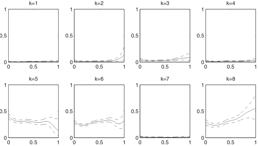
To demonstrate the practical utility of the proposed VNB method, we consider a MPH dataset. More specifically, the dataset used consists 13,613 documents from m=8 different functional departments with p=4,778 keywords. All of the observations are collected between 8:00 AM and 24:00 PM. Then, the recording time are standardized to [0,1]. Half of these documents (i.e., n=6806) are selected randomly for training whereas the remainder are used for testing. At each testing recording time, all parameters of the VNB model are estimated by kernel estimators (2.2) and (2.3) based on the training data. To visualize the time-varying pattern, the estima-tors{πkˆ (u) : 1≤k≤8}with their 90% confidence bands based on 1000 bootstrap replications of the training set are plotted in
Figure 1. Similarly, the time-varying pattern of ˆθkj(u) can also be obtained in the same manner (e.g., seeFigure 2). These two figures show that the confidence bands become larger asutends to 1. That’s because events are likely to happen in the daytime and less likely to happen at midnight, which results in the effec-tive sample sizes becoming smaller asutends to 1. Thus, such a
0 0.5 1 0
0.1 0.2 0.3 0.4
k=1
0 0.5 1 0
0.1 0.2 0.3 0.4
k=2
0 0.5 1 0
0.1 0.2 0.3 0.4
k=3
0 0.5 1 0
0.1 0.2 0.3 0.4
k=4
0 0.5 1 0
0.1 0.2 0.3 0.4
k=5
0 0.5 1 0
0.1 0.2 0.3 0.4
k=6
0 0.5 1 0
0.1 0.2 0.3 0.4
k=7
0 0.5 1 0
0.1 0.2 0.3 0.4
k=8
Figure 1. {πˆk(u) : 1≤k≤8}(solid lines) together with their 90% confidence bands (dashed lines) based on 1000 bootstrap replications of the training set are plotted. The time-varying pattern can be clearly obtained.
time-dependent classification method should be more practical for this type of data. We then apply the proposed BIC method to the training set and 489 keywords are selected as relevant features. Based on these selected keywords, a VNB classifier is estimated and its misclassification error (ME) is evaluated based on the testing set. For comparison’s sake, ME values of full model based KNN, AdaB, RF, SVM, NB, and VNBπare also included. Alternatively, a simple way to deal with the
record-ing time is to include it directly as the (p+1)th feature (i.e., Xi,p+1=Ui, particularly setXi,p+1=I(Ui > n−1
iUi) for NB). Its actual performance is evaluated on various methods except VNBπ and VNB. The detailed results are summarized inTable 3. As one can see, VNBπ performs better than NB, which confirms that the class probabilities{πkˆ (u) : 1≤k≤8} are truly time-varying. In addition, VNB performs best and im-proves the prediction accuracy further.
0 0.5 1 0
0.5 1
k=1
0 0.5 1 0
0.5 1
k=2
0 0.5 1 0
0.5 1
k=3
0 0.5 1 0
0.5 1
k=4
0 0.5 1 0
0.5 1
k=5
0 0.5 1 0
0.5 1
k=6
0 0.5 1 0
0.5 1
k=7
0 0.5 1 0
0.5 1
k=8
Figure 2. {θˆkj1(u) : 1≤k≤8}(solid lines) together with their 90% confidence bands (dashed lines) based on 1000 bootstrap replications of
the training set are plotted, wherej1=argmaxj∈M{
k
iπˆk[ ˆθkj(Ui)−θˆkj]2}. Different time-varying patterns are clearly obtained.
Table 3. Results of MPH Example
Classification methods KNN AdaB RF SVM NB VNBπ VNB
ME(%) based onpfeatures 23.58 36.99 6.07 29.19 6.77 5.83 5.32
ME(%) based onp+1 features 26.47 36.99 6.76 29.15 6.76 – –
4. CONCLUDING REMARKS
In this study, we developed a novel method, VNB, for Chinese document classification. This new method can be viewed as a natural extension of the classical NB method but with a much improved modeling capability. Nonparametric kernel method was used to estimate the unknown parameters and a BIC-type screening criterion (Wang and Xia2009) was used to select im-portant features. The excellent performance of the new method was confirmed by both simulated data and the MPH datasets. To conclude the article, we identify two interesting topics for future study.
First, the current VNB model only handles a univariate index variable. In a more complex situation, it is likely to have a multi-variate index variable. For example, in addition to the recording time, the demographic information (e.g., age and gender) related to the caller can also be collected. This generates a multivariate index variable. In this case, modelingπk(u) andθkj(u) directly as fully nonparametric functions inuis unlikely to be the opti-mal choice. Thus, various semiparametric models might be more preferable, for example, varying coefficient models (Hastie and Tibshirani1993; Cai, Fan, and Li2000), single index models (Xia2006; Kong and Xia 2007), and partially linear models (H¨ardle, Liang, and Gao2000; Fan and Huang2005).
Second, the current VNB model assumes that every feature has time-varying effect. In fact, it is likely that the effects of some features do not change according to time. Thus, there might exist some featurej, such thatθkj(u)=θkj for every 1≤k≤mand 0≤u≤1. We then define
μj = m
k=1
πkE{θkj(Ui)−θkj}2.
Accordingly,{θkj(u) : 1≤k≤m}are constant functions, if and only ifμj =0. Next, we define a varying model asV= {1≤ j ≤p:μj >0}. In practice,μj can be estimated by
ˆ μj =n−1
m
k=1
n
i=1 ˆ
πk{θkjˆ (Ui)−θkjˆ }2.
Thus, the varying model can be estimated as V = {1≤j ≤ p: ˆμj > ξ}for someξ >0. Theoretically, we can prove that P(V =V)→1 as n→ ∞, ifξ is selected in an appropriate manner. However, the practical selection ofξis still an ongoing research project. Further research is needed in this direction.
APPENDIX A. TECHNICAL CONDITIONS
To investigate the asymptotic properties of the proposed VNB method, the following technical conditions are needed.
(C1) (Kernel Assumption) K(t) is a symmetric and bounded density function, with finite second-order moment and bounded first-order derivative onR1.
(C2) (Smoothness Assumption) πk(u), θkj(u) and f(u) have bounded first-order and second-order derivatives on [0,1], for allkandj, wheref(u) is the density function ofUi. (C3) (Dimension Assumption)The true model size is assumed
to be 1≤ |MT| ≤n, and logp∝nξ for some 0< ξ < 3/5, asn→ ∞.
(C4) (Boundedness Assumption) There exist some positive constants fmax and ν <min{1/m,1/3}, such that ν≤
f(u)≤fmax, πk(u)≥ν andν≤θkj(u)≤1−ν, for all
k, j and u∈[0,1]. Moreover, for j ∈MT, there ex-ist some k∈ {1, . . . , m}and some set Skj ⊂[0,1] with measure no less than some positive constantτ, such that infu∈Skj|θkj(u)−θj(u)| ≥ν.
Both conditions (C1) and (C2) are quite standard and have been used extensively in existing literature (Fan and Gijbels1996; Li and Racine2006). Under these assumptions, we have ˆf(u)= n−1iKh(Ui−u)→p f(u), ˆπk(u)→p πk(u) and ˆθkj(u)→p θkj(u), as long ash→0 andnh→ ∞. Condition (C3) gives us the exponential divergence speed of p, as n→ ∞. Under condition (C4), we can see clearly that minj∈MTφj >0 and
φj =0 forj /∈MT. Thus, all relevant features are apart from the irrelevant ones, which can be identified consistently based on the appropriate critical valuec.
APPENDIX B. A TECHNICAL LEMMA
Lemma B.1. Let 0< ν <1/3, then there exists a positive constantC(depending onν), the following inequality holds,
inf
ν≤A≤1−ν,ν≤B≤1−ν,|A−B|≥ν
AlogA
B +(1−A) log 1−A 1−B
≥C.
(B.1)
Proof. By Jensen’s inequality, it is clear thatAlogA B+(1− A) log1−A
1−B ≥0, and the equality holds if and only ifA=B. Now, we consider a binary function g(x, y)=xlogxy+(1− x) log11−−xy, wherex, y∈[ν,1−ν] and|x−y| ≥ν. Then, we can easily obtain the first-order and second-order partial deriva-tives ofgwith respect toy,
∂g ∂y =
y−x y(1−y),
∂2g
∂y2 =
x−2xy+y2
y2(1−y)2 >
x2−2xy+y2
y2(1−y)2 >0. It follows that, givenx,g(x, y) is a convex function ofyand reaches its minimum at y =x+ν or x−ν. Next, consider two functionsg(x, x+ν) withx ∈[ν,1−2ν] andg(x, x−ν) with x ∈[2ν,1−ν], which have the same minimum. With-out loss of generality, we may only care abWith-out the continuous
function g(x, x+ν). Thus, there exists some x0∈[ν,1− 2ν], such thatg(x0, x0+ν)=minx∈[ν,1−2ν]{g(x, x+ν)}. Re-call Jensen’s inequality,g(x0, x0+ν)>0 is obvious. Finally, takingC =g(x0, x0+ν), inequality (B.1) holds.
APPENDIX C. PROOF OF THEOREM 1
To prove the theorem, it suffices to show that maxj|φjˆ − hand side of (C.1) converges to 0 in probability. Thus, the uni-form consistency of ˆφj is implied by the following important conclusions (for a fixedk):
max
These conclusions would be proved in details subsequently. Step 1. We first consider (C.2) and (C.3). Under the technical conditions (C1)–(C3), one can verify that (C.2) and (C.3) are implied by the following three conclusions:
sup
Because the proof techniques are similar, we would only provide details for (C.5). To this end, we define uv =v/N for v= identically distributed random variables taking values in a bounded interval [0, h−1M
1], where M1=supt∈R1K(t)<∞
by condition (C1). Thus we have|Wi−E{Wi}| ≤h−1M1 and var(Wi)=E[Wi−E{Wi}]2≤h−2M12. Based on these facts, we apply the Bernstein’s inequality (Lin and Bai 2010) and obtain
We then consider the right-hand side of (C.7), (C4). The detailed proof of inequality (C.12) can be found in existing literature (Li and Racine2006). Note that|ZikXij| ≤1 ilarly, by condition (C2), one can verify that the right-hand side of (C.9) is upper bounded byN−1M3for some positive constant right-hand side of (C.14) are equal to 0 for sufficiently largen. Therefore, under the condition (C3) and assumen→ ∞, we have the right-hand side of (C.14) converges toward 0.
Step 2. We next consider (C.4). Define a statistic Ti =
{θkj(Ui)−θj(Ui)}2, which is a nonparametric function ofUi. It
is clear that{Ti : 1≤i≤n}are independent and identically dis-tributed random variables taking values in interval [0,1]. Then, we have |Ti−E{Ti}| ≤1 and var(Ti)=E[Ti−E{Ti}]2≤1. Based on these facts, the Bernstein’s inequality can be used immediately,
Next, by Bonferroni’s inequality, we have
P
Then by condition (C3), we know that the right-hand side of (C.15) converges toward 0. This completes the entire proof.
APPENDIX D. PROOF OF THEOREM 2
According to Theorem 1, after given technical conditions (C1)–(C4) and some appropriate critical value c, we must haveP(MT ∈M)→1. It implies thatP(M(d0) =MT)→1,
whered0 = |MT|is the true model size. To prove Theorem 2, the following inequality should be needed:
P(MT ⊂M)
proof is divided into the following three steps.
Step 1. We start with the difference of BIC values between two models as
For simplicity, some tedious manipulation of (D.1) is omitted. Next, define a nonparametric functionGj(u) as
Gj(u)= Step 2. The next thing to prove is the consistency result n−1n
l=1Gˆj(Ul)→p E{Gj(U1)} for everyj. By triangle in-equality, it can be implied by the following two conclusions:
sup
Now, we provide some details for (D.2) first. After some tedious manipulation, we get the following equalities, for fixed jandu∈[0,1]. it’s not difficult to get the following exponential inequality un-der conditions (C1), (C2), and (C4). Givenk(1≤k≤2m), for any >0 and sufficiently largen,
P
whereC1andC2are some positive constants. Because the proof techniques are similar but not particularly difficult, the detailed proof of (D.4) will not be reproduced here. For a givenu, define g(A)Gjˆ (u) andg(a)Gj(u), whereA=(A1, . . . , A2m)
By Bonferroni’s inequality, the right-hand side of (D.7) can be further bounded by
Together with inequality (D.4) andmis a finite number, we can get the following uniform consistency result. For any 0< ≤ 2−1M4ν3and sufficiently largen,
whereC3andC4are some positive constants.
We next provide a detailed proof for (D.3). By condition (C4), it is clear that|Gj(Ul)−E{Gj(U1)}|< M5and var{Gj(Ul)} ≤
M52, where M5=fmax(1−ν){log(1−ν)−logν}. Based on these facts, the Bernstein’s inequality can be used,
P
for any >0. Thus, combining the conclusions of (D.8) and (D.9), for any 0< ≤2−1M
4ν3 and sufficiently large n, the
following inequality holds, whereC5andC6are some positive constants.
Step 3. For simplicity, we use the notationS=M(d0)\M(d)
throughout the rest of proof. According to Equation (D.1), we immediately know that ciently largen, the probability (D.11) can be bounded by
≤P
Then by Bonferroni’s inequality, the right-hand side of (D.12) can be bounded by
≤P Under the assumptiond0≤n, as given in condition (C3), the right-hand side of (D.14) converges toward 0, as n→ ∞. Consequently, we haveP(BIC(M(d))>BIC(M(d0)))→1 for
M(d) ⊂M(d0)=MT. This completes the third step and
fin-ishes the entire proof.
ACKNOWLEDGMENTS
Guan and Guo’s research was supported in part by the Na-tional Natural Science Foundation of China (No. 11025102), Natural Science Foundation of Jilin Province (No. 20100401), Program for Changjiang Scholars and Innovative Research Team in University. Wang’s research was supported in part by National Natural Science Foundation of China (No. 11131002
and No. 11271032), Fox Ying Tong Education Foundation, the Business Intelligence Research Center at Peking University, and the Center for Statistical Science at Peking University.
[Received May 2013. Revised February 2014.]
REFERENCES
Biau, G., Devroye, L., and Lugosi, G. (2008), “Consistency of Random Forests and Other Averaging Classifiers,”Journal of Machine Learning Research, 9, 2015–2033. [445]
Blei, D. M., Ng, A. Y., and Jordan, M. I. (2003), “Latent Dirichlet Allocation,” Journal of Machine Learning Research, 3, 993–1022. [446]
Breiman, L. (2001), “Random Forests,”Machine Learning, 45, 5–32. [445] Breiman, L., Friedman, J. H., Olshen, R. A., and Stone, C. J. (1998),
Classifi-cation and Regression Trees, New York: Chapman & Hall/CRC. [445] Buhlmann, P., and Yu, B. (2003), “Boosting with the L2 Loss: Regression and
Classification,”Journal of the American Statistical Association, 98, 324– 340. [445]
Cai, Z., Fan, J., and Li, R. (2000), “Efficient Estimation and Inferences for Varying-Coefficient Models,”Journal of the American Statistical Associa-tion, 95, 888–902. [451]
Fan, J., and Fan, Y. (2008), “High-Dimensional Classification Using Features Annealed Independence Rules,”The Annals of Statistics, 36, 2605–2637. [445]
Fan, J., and Gijbels, I. (1996),Local Polynomial Modeling and Its Applications, New York: Chapman & Hall. [446,451]
Fan, J., and Huang, T. (2005), “Profile Likelihood Inferences on Semiparametric Varying-Coefficient Partially Linear Models,”Bernoulli, 11, 1031–1057. [451]
Fan, J., and Li, R. (2001), “Variable Selection via Nonconcave Penalized Like-lihood and Its Oracle Properties,”Journal of the American Statistical Asso-ciation, 96, 1348–1360. [448]
Fan, J., and Lv, J. (2008), “Sure Independence Screening for Ultra-High Di-mensional Feature Space,”Journal of the Royal Statistical Society,Series B, 70, 849–911. [446,447]
H¨ardle, W., Liang, H., and Gao, J. (2000),Partially Linear Models, Heidelberg: Springer. [451]
Hastie, T. J., and Tibshirani, R. J. (1993), “Varying-Coefficient Models,”Journal of the Royal Statistical Society,Series B, 55, 757–796. [451]
Hastie, T., Tibshirani, R., and Friedman, J. (2001),The Elements of Statistical Learning, New York: Springer. [445]
Johnson, R. A., and Wichern, D. W. (2003),Applied Multivariate Statistical Analysis(5th ed.), New York: Pearson Education. [445]
Kong, E., and Xia, Y. (2007), “Variable Selection for Single-Index Model,” Biometrika, 94, 217–229. [451]
Lee, D. L., Chuang, H., and Seamons, K. (1997), “Document Ranking and the Vector-Space Model,”Software, IEEE, 14, 67–75. [445]
Leng, C. (2008), “Sparse Optimal Scoring for Multiclass Cancer Diagnosis and Biomarker Detection Using Microarray Data,”Computational Biology and Chemistry, 32, 417–425. [445]
Lewis, D. D. (1998), “Na¨ıve Bayes at Forty: The Independence Assumption in Information Retrieval,”Proceedings of ECML-98, 10th European Confer-ence on Machine Learning, 4–15. [445,446]
Li, Q., and Racine, J. S. (2006), Nonparametric Econometrics, Princeton: Princeton University Press. [447,451,453]
Lin, Z., and Bai, Z. (2010),Probability Inequalities, Beijing: Science Press. [452]
Liu, Y., Zhang, H. H., and Wu, Y. (2011), “Hard or Soft Classification? Large-Margin Unified Machines,”Journal of the American Statistical Association, 106, 166–177. [445]
Mai, Q., Zou, H., and Yuan, M. (2012), “A Direct Approach to Sparse Discrim-inant Analysis in Ultra-High Dimensions,”Biometrika, 99, 29–42. [445] Manevitz, L. M., and Yousef, M. (2001), “One-Class SVMs for Document
Classification,”Journal of Machine Learning Research, 2, 139–154. [445] Murphy, K. P. (2012),Machine Learning: A Probabilistic Perspective,
Cam-bridge, MA: The MIT Press. [445]
Qiao, X., Zhang, H. H., Liu, Y., Todd, M. J., and Marron, J. S. (2010), “Weighted Distance Weighted Discrimination and Its Asymptotic Properties,”Journal of the American Statistical Association, 105, 401–414. [445]
Ramsay, J. O., and Silverman, B. W. (2005),Functional Data Analysis(2nd ed.), New York: Springer. [445]
Ripley, B. D. (1996),Pattern Recognition and Neural Networks, New York: Cambridge University Press. [445]
Salton, G., and McGill, M. (1983),Introduction to Modern Information Re-trieval, New York: McGraw-Hill. [446]
Shao, J., Wang, Y., Deng, X., and Wang, S. (2011), “Sparse Linear Discimi-nant Analysis by Thresholding for High Dimensional Data,”The Annals of Statistics, 39, 1241–1265. [445]
Wang, H. (2009), “Forward Regression for Ultra-High Dimensional Variable Screening,”Journal of the American Statistical Association, 104, 1512– 1524. [446,447]
Wang, H., and Xia, Y. (2009), “Shrinkage Estimation of the Varying Coefficient Model,”Journal of the American Statistical Association, 104, 747–757. [447,451]
Wang, L., Zhu, J., and Zou, H. (2006), “The Doubly Regularized Support Vector Machine,”Statistica Sinica, 16, 589–616. [445]
Wu, X., and Kumar, V. (2008), “The Top Ten Algorithms in Data Mining,” Knowledge and Information Systems, 14, 1–37. [446]
Wu, Y., and Liu, Y. (2007), “Robust Truncated-Hinge-Loss Support Vector Machines,”Journal of the American Statistical Association, 102, 974–983. [445]
——— (2013), “Functional Robust Support Vector Machines for Sparse and Ir-regular Longitudinal Data,”Journal of Computational and Graphical Statis-tics, 22, 379–395. [445]
Xia, Y. (2006), “Asymptotic Distributions of Two Estimators of the Single-Index Model,”Econometric Theory, 22, 1112–1137. [451]
Zhang, H. H. (2006), “Variable Selection for Support Vector Machines via Smoothing Spline ANOVA,”Statistica Sinica, 16, 659–674. [445] Zhu, J., Zou, H., Rosset, S., and Hastie, T. (2009), “Multi-Class Adaboost,”
Statistics and Its Interface, 2, 349–360. [445]
Zou, H., Zhu, J., and Hastie, T. (2008), “New Multicategory Boosting Algo-rithms Based on Multicategory Fisher-Consistent Losses,”The Annals of Applied Statistics, 2, 1290–1306. [445]