Full Terms & Conditions of access and use can be found at
http://www.tandfonline.com/action/journalInformation?journalCode=ubes20
Download by: [Universitas Maritim Raja Ali Haji] Date: 11 January 2016, At: 19:18
Journal of Business & Economic Statistics
ISSN: 0735-0015 (Print) 1537-2707 (Online) Journal homepage: http://www.tandfonline.com/loi/ubes20
Flexible Modeling of Dependence in Volatility
Processes
Maria Kalli & Jim Griffin
To cite this article: Maria Kalli & Jim Griffin (2015) Flexible Modeling of Dependence in Volatility Processes, Journal of Business & Economic Statistics, 33:1, 102-113, DOI: 10.1080/07350015.2014.925457
To link to this article: http://dx.doi.org/10.1080/07350015.2014.925457
Accepted author version posted online: 12 Jun 2014.
Submit your article to this journal
Article views: 193
View related articles
Flexible Modeling of Dependence in Volatility
Processes
Maria KALLI
Business School, Canterbury Christ Church University, North Holmes Road, Canterbury CT1 1QU, United Kingdom ([email protected])
Jim GRIFFIN
School of Mathematics, Statistics and Actuarial Science, University of Kent, Canterbury CT2 7NF, United Kingdom ([email protected])
This article proposes a novel stochastic volatility (SV) model that draws from the existing literature on autoregressive SV models, aggregation of autoregressive processes, and Bayesian nonparametric modeling to create a SV model that can capture long-range dependence. The volatility process is assumed to be the aggregate of autoregressive processes, where the distribution of the autoregressive coefficients is modeled using a flexible Bayesian approach. The model provides insight into the dynamic properties of the volatility. An efficient algorithm is defined which uses recently proposed adaptive Monte Carlo methods. The proposed model is applied to the daily returns of stocks.
KEY WORDS: Aggregation; Bayesian nonparametric; Dirichlet process; Long-range dependence; MCMC; Stochastic volatility.
1. INTRODUCTION
Stochastic volatility (SV) models have become a popular method for modeling financial data. The SV model described in Taylor (1986) and Harvey (1998) assumes that returns,yt, are modeled by
yt =βexp{ht/2}ǫt, t=1,2, . . . , T , (1)
whereǫtare iid draws from some distribution (usually, taken to be normal) and exp{ht/2}is the volatility on thetth day which is assumed to follow a stochastic process. This volatility process can be thought to represent the flow of information to the market and log volatility is often assumed to follow an AR(1) process
ht=φht−1+ηt, t=1,2, . . . , T , (2)
where ηt is normally distributed with mean 0 and variance
σ2(1−φ2). This choice of distribution forηt results in the sta-tionary distribution ofhtbeing normal with mean 0 and variance
σ2.The autoregressive coefficient ofh
t−1,φ, is the persistence
parameter measuring the first lag autocorrelation ofht.
The AR(1) assumption has become standard, but there are no overriding economic reasons for its choice. Empirical analyses of financial return series have suggested that the volatility pro-cess is time-varying and mean-reverting with volatility cluster-ing, for a comprehensive description of these stylized facts see, for example, Cont (2001), Tsay (2005), and Taylor (2005). These analyses have also observed that the rate of decay of the sample autocorrelation function of the squared and absolute returns is much slower than would be expected with an AR(1) volatility process. The slow decay of the sample autocorrelation function has been linked to the concept of long-range dependence. We are interested in the case whereht is the aggregate of weakly stationary processes, with a clearly defined covariance func-tion (and thus spectral density). Then, long-range dependence occurs when this covariance function is unsummable (see
Granger1980). Alternatively, whenht is a stationary process, long-range dependence can be defined in terms of fractional dif-ferencing. A process has long-range dependence if the spectral densityS(ω) converges toκ|ω|−2dat very low frequencies, that is, asω→0, where the differencing parameterd ∈(0,1/2) and
ω∈[−π, π].
Early evidence of the slow rate of decay of the sample auto-correlation function in financial time series can be traced back to Ding et al. (1993), De Lima and Grato (1994), and Bollerslev and Mikkelsen (1996). Ding et al. (1993) constructed a series of fractional moments using the daily returns of the S&P 500 and found very slowly decaying autocorrelations for these series, De Lima and Grato (1994) applied some long memory tests to the squared residuals of filtered daily U.S. stock returns and rejected the null hypothesis of short memory for these returns. Bollerslev and Mikkelsen (1996) found slowly decaying autocorrelations for the absolute returns of the S&P 500 and proposed the frac-tionally integrated GARCH (FIGARCH) as well as the fraction-ally integrated EGARCH (FIEGARCH). In terms of modeling long-range dependence in SV models (LMSV), Harvey (1998) proposed an SV model driven by fractional noise where the log volatility ht is expressed as a simple autoregressive
frac-tionally integrated moving average, ARFIMA(0, d,0). Breidt, Grato, and De Lima (1998) extended this model by expressing the log volatility,ht as an ARFIMA(p, d, q). Generalizations of the LMSV appear in Arteche (2004) and Hurvich, Moulines, and Soulier (2005), where the Gaussianity assumption forhtis replaced by a linearity assumption in both cases. The authors use the results in Surgailis and Viano (2002), and confirm that under linearity forht and other weak assumptions, powers of absolute returns have long-range dependence.
© 2015American Statistical Association Journal of Business & Economic Statistics
January 2015, Vol. 33, No. 1 DOI:10.1080/07350015.2014.925457
102
Cross-sectional aggregation of AR(1) processes was intro-duced in Robinson (1978) and further explored in Granger (1980) and Zaffaroni (2004). The aggregation of such processes leads to a class of models with long-range dependence which differ from fractionally integrated models, where the series re-quires fractional differencing to achieve a stationary ARMA series.
Suppose that we havemtime serieshi,1, hi,2, . . . , hi,T fori=
1, . . . , mof the form
hi,t =φihi,t−1+ηi,t, (3)
whereηi,t∼N(0, σ2(1−φi2)) are idiosyncratic shocks, and the
persistence parameterφi∼iidFφ, with support on (0,1). The ag-gregate process is
Granger (1980) studied the effect of the distributional choice of Fφ on the properties and the dependence structure of the aggregate. He showed that the aggregate has the spectrum of an ARMA(m, m−1) ifFφis discrete withmatoms on region (−1,1). If Fφ is continuous and φ can take on any value on some region in (−1,1), then the spectrum of the aggregate does not have the form of an ARMA spectrum. He observed that the behavior of fφ, the density ofFφ, is important when φ≈1,
because it has an effect on long-range dependence. He assumed that Fφ is a beta distribution on (0,1) with shape parameters
a and b, and confirmed that the key parameter, in terms of long-range dependence, isb. He showed that whenb→ ∞the autocovariance function of the aggregate approximates that of an ARMA process. Zaffaroni (2004) generalized the results of Granger (1980) to distributions with densityfφ(φ)∝g(φ)(1−
φ)bon (0,1) and considers the limit of the processht/√var [ht].
rather than the limit of its autocorrelation function. He showed that the process is stationary ifb >0 but nonstationary ifb <0. This article describes a Bayesian nonparametric approach to estimating the distributionFφ. Bayesian nonparametric models place a prior on an infinite-dimensional parameter space and adapt their complexity to the data. A more appropriate term is infinite capacity models, emphasizing the crucial property that they allow their complexity (i.e., the number of parameters) to grow as more data are observed; in contrast, finite-capacity models assume a fixed complexity. Hjort et al. (2010) is a recent book length review of Bayesian nonparametric methods. The distributionFφ is assumed to be discrete which allows us to
decompose the aggregate process into processes with different levels of dependence. This models the effect of uneven informa-tion flows on volatility and can be linked to the differences in effects of different types of information. Some information may have a longer lasting effect on volatility than other pieces of in-formation. A similar approach was discussed by Griffin (2011) using continuous time non-Gaussian Ornstein–Uhlenbeck pro-cesses for the volatility. Inference is made using Markov chain Monte Carlo (MCMC) methods with a finite approximation to the well-known Dirichlet process which exploits the relationship between the Dirichlet and gamma distributions, see Ishwaran and Zarepour (2000,2002). The offset mixture representation of the SV model (Kim, Shephard, and Chib,1998) allows us to
jointly update the volatilities using the forward filtering back-wards sampling algorithm of Fr¨uhwirth-Schnatter (1994) and Carter and Kohn (1994). This combined with recently devel-oped adaptive MCMC methodology enables us to construct an efficient MCMC algorithm for these models.
The structure of this article is as follows. In Section 2, we describe in detail the use of Bayesian nonparametric priors in aggregation models, Section3describes our sampling method-ology, in Section4we provide illustrations with both simulated and real data, Section5is the discussion.
2. BAYESIAN NONPARAMETRIC INFERENCE IN AGGREGATION MODELS
The core of Bayesian nonparametrics is placing a prior on an infinite-dimensional parameter space. In our context, the pa-rameter is a probability distribution and the prior is a stochastic process. We will define a Bayesian nonparametric model for cross-sectional aggregation models in two stages. First, we con-struct a suitable limiting process for a cross-sectional aggrega-tion model as the number of elements tends to infinity. Second, we discuss the use of a Dirichlet process prior (Ferguson1973) forFφ, the distribution of the persistence parameterφ.
We use the notationht(φ, σ2) to represent an AR(1) process with persistence parameterφand stationary varianceσ2so
ht(φ, σ2)=φht−1(φ, σ2)+ηt,
whereηt ∼N(0, σ2(1−φ2)),and so the marginal distribution ofht(φ, σ2) is N(0, σ2). We define the aggregate in (4) as:
Definition 1. A finite cross-sectional aggregation (FCA) pro-cessh(tm)with parametersm,σ2, andFφis defined by
The stationary distribution of the FCA process isN(0, σ2/m) and the autocorrelation function,ρs=corr (h(tm), h
(m)
t+s), has the
formρs =EFφ[φ
s] if it exists.
In the introduction, we stressed the importance of the persis-tence parameter distribution,Fφ, in determining the dependence structure of the FCA process. To find a suitable limit for h(tm)
asm→ ∞, we will assume thatFφ is discrete with an infinite number of atoms, such that
Fφ=
the Dirac measure placing mass 1 at locationλj. This assump-tion means that no long memory is present, although arbitrary levels of long-range dependence exist.
The valuesφ1, . . . , φmin the FCA process are sampled from Fφ and, since it is a discrete distribution, eachφi must take a
value in λ1, λ2, . . . and there can be ties in these values. We
letn(jm) be the number ofφi’s which are equal toλj. Clearly
n(1m), n(2m), . . . will follow an infinite-dimensional multinomial
distribution which depends onm. It follows that, with this choice
and its stationary distribution isN(0,1) since this distribution does not depend onm. It is useful to have a scaled version of this limit for our modeling purposes which we call an ICA process.
Definition 2. An infinite cross-sectional aggregation (ICA) processh(t∞)with parametersσ2andFφis defined by
The distribution of Fφ which defines the ICA process has a natural interpretation aswj is the proportion of the variation in the stationary distribution explained by thejth process which is associated with AR parameterλj. The spectral density,S(ω), can also be expressed as an integral with respect toFφ,
S(ω)=σ2
1
(1−λ2)(1+λ2−2λcos(ω))dFφ(λ),
where (1−λ2)(1+λ12−2λcos(ω)) is the spectral density of an AR(1)
process with persistence parameterλand marginal variance 1. Our focus is on the estimation ofFφ. To avoid making para-metric assumptions about this distribution, we take a Bayesian nonparametric approach and use a Dirichlet process (DP) prior forFφ. The DP prior is often used to define an infinite mixture model for density estimation by giving the mixing distribution a DP prior. Our approach is substantially different and uses the Dirichlet process as prior for the distribution Fφ in the ICA
process model. This leads to a nonparametric approach to un-derstanding the dynamic behavior of the aggregateh(t∞).
The properties and theory for the DP were developed in Fer-guson (1973). We say that a random distributionFwith sample spaceis distributed according to a DP if the masses placed on all partitions ofare Dirichlet distributed. To elaborate, let
F0 be a distribution over sample spaceandca positive real
number, then for any measurable partitionA1, . . . , Arofthe
vector (F(A1), . . . , F(Ar)) is random sinceF is random. The
Dirichlet process can be defined as
F ∼DP(c, F0) if
(F(A1), . . . , F(Ar)) (9)
∼Dir(cF0(A1), . . . , cF0(Ar))1
for every finite measurable partitionA1, . . . , Ar of.
The distributionF0is referred to as the centering distribution
as it is the mean of the DP, that is E[F(Ai)]=F0(Ai). The
positive numbercis referred to as the concentration (or preci-sion) parameter as it features in and controls the variance of the DP, that is var[F(Ai)]=F0(Ai)(1−F0(Ai))/(c+1).One can
clearly see that the larger the value ofc, the smaller the vari-ance, and hence the DP will have more of its mass concentrated around its mean.
We now describe the priors given to the parameters of the ICA process. The distributionFφ is given a Dirichlet process prior with precision parametercand a Be(1, b) centering distribution. The parameterσ2∼Ga(c, c/ζ) where Ga(α1, α2) represents a a Dirichlet process prior forFφ implies that this distribution is a priori discrete with probability 1 and so it is suitable for use with the ICA process. An alternative parameterization of theFφ
is
A SV with ICA volatility process (SV-ICA) model can now be defined for returnsy1, . . . , yT
t follows an ICA process. This model
allows a flexible form for the autocorrelation and helps de-composition of the volatility process dynamics. The model is completed by specifying priors for the parametersβ, b, c, and
ζ. The parameterμ=logβ2 is given a vague improper prior,
p(μ)∝1.This makes the prior invariant to rescaling of the data. The hyperprior ofb, the scale parameter of the distribution ofλi, is taken to be an exponential distribution with mean 1/(log 2). This implies that the prior median ofbis 1 and hence places half
1Dir(α
1, α2, . . . , αk+1) represents thek-dimensional Dirichlet distribution.
its mass on the processes with long memory and half its mass on processes with short memory. This choice avoids making strong assumptions about the dynamic properties of the time series. The parameterccontrols how closeFφis to the beta centering distribution. We follow Griffin and Steel (2004) by defining the prior forcthrough c
c+n0 ∼Be(ac, ac), wheren0is a prior sample
size forFφandacis a precision parameter (smaller values ofac
imply less variability). The density forcis
p(c)=n
the mass on relatively small values ofcimplying thatFφis away from the beta distribution. The parameterζ represents the prior mean of the overall variabilityσ2 of the volatility process. We represent our prior ignorance about this scale by choosing the vague priorζ−1
∼Ga(0.001,0.001).
3. COMPUTATION
Markov chain Monte Carlo (MCMC) inference in the SV-ICA model is complicated by the presence of an infinite sum of AR(1) processes and the nonlinear state space form of the model. The first problem is addressed through a finite truncation ofFφand the second problem through the offset mixture representation of the SV model discussed in Kim, Shephard, and Chib (1998), Omori et al. (2007), and Nakajima and Omori (2009).
The approximation of the Dirichlet process by finite trunca-tions has been discussed by many authors including Neal (2000), Richardson and Green (2001), Ishwaran and Zarepour (2000), and Ishwaran and Zarepour (2002). In the latter article, the au-thors discussed using Dirichlet random weights to construct a finite-dimensional random probability measure with n atoms that limits to a Dirichlet process as n→ ∞. Their approach approximatesFφ by
Be(1, b). The relationship between the Dirichlet distribution and the gamma distribution allows us to further write
Fφ(n) =
Ga(c, c/ζ), replicating the prior for the infinite-dimensional model. The idea of using Gamma priors for variances to avoid model overcomplexity has been explored recently in the Bayesian literature on regression models (see Caron and Doucet
2008, and Griffin and Brown2010).
Combining the finite truncationFφ(n)ofFφ with the SV-ICA model leads to the model (where we drop the dependence of the model on the value ofnfor notational simplicity)
yt =βexp{ht/2}ǫt, ht= We proceed to inference using the linearized form of the SV model for MCMC (Kim et al.1998; Omori et al.2007; Nakajima and Omori2009). This approach works withy∗
t =log(yt2+ξ),
where the offset valueξ is introduced to avoidy∗
t from being
very negative or even undefined, due to zero returns, see Fuller (1996). It follows thaty∗
t can be expressed as a linear function
ofht,
yt∗=μ+ht+ǫt∗ t =1, . . . , T , (13)
where μ=log(β2),ǫ∗t =log(ǫt2) andǫt∗ follows a logχ2 dis-tribution. The logχ2 distribution can be approximated by a
mixture of seven normal distributions
p(ǫt∗)=
The SV-ICA model with the finite truncation ofFφ and the
linearized form for the return defines a Gaussian dynamic linear model conditional ons1, s2, . . . , sT andσ12, σ22, . . . , σn2,
y∗
t and ht is a linear, Gaussian state-space model and so the
marginal likelihoodp(y∗
1, . . . , yT∗|θ) can be calculated
analyti-cally using the Kalman filter andθupdated using Metropolis-Hastings random walk steps. This approach, however, has some problems. The value ofnwill often be large and the number of computations needed to calculate the marginal likelihood will be
O(n3) (due to the matrix inversions involved). This makes this scheme only computationally feasible whennis small (say, less than 10). It would also be difficult to propose a high-dimensional vector of new parameter values. On the other hand, the param-eters can be sampled using a Gibbs sampler by simulating the hidden stateshi,t using a forward filtering backward sampling
(FFBS) algorithm, (Carter and Kohn1994; Fr¨uhwirth-Schnatter
1994). However, this sampler is known to mix slowly whenλj
becomes close to 1.
We propose an algorithm which combines both samplers. The parameters are updated using the Gibbs sampler. Additional steps are added which choosek < ncomponents and update pa-rameters conditional on the states of the other components while marginalizing over the states in thekcomponents (we usek=4 in our examples). This set up allows us to improve the poor mixing associated with the Gibbs sampler while controlling the computational cost. The sampler uses adaptive proposals, which are allowed to depend on previous values of the sampler, in a Metropolis-within-Gibbs scheme. These schemes destroy the Markovian structure of the sampler and so special theory must be developed to prove convergence of these algorithms to the correct stationary distribution. Convergence of Metropolis-within-Gibbs scheme was discussed by Haario, Saksman, and Tamminen (2005), Roberts and Rosenthal (2009), and Latuszyn-ski, Roberts, and Rosenthal (2013). In particular, we assume that the parametersσ12, . . . , σn2,candbare truncated at large values, which ensures uniform ergodicity of the chain and ergodicity of the chain follows from Theorem 5.5 of Latuszynski, Roberts, and Rosenthal (2013). It will be useful to definex(m) to be the value of some parameterxat the start of themth iteration. The steps of the sampler are:
Updatingσ12, σ22, . . . , σn2. The full conditional distribution
where GIG(a1, a2, a3) represents the generalized inverse
Gaus-sian distribution which has density proportional to
ya1−1exp
which is updated using a random walk on the logit scale (i.e., the proposal value at the mth iteration λ′
j is simulated
The tuning parameterσλ,j2 (m) is updated in the sampler so that the acceptance rate converges to 0.3 (following the advice of Roberts and Rosenthal (2009) using the method of Atchad´e and Rosenthal (2005)). This involves setting
σλ,j2 (m+1)=ρσλ,j2 (m)+m−0.6(α−0.3)
,
whereαis the acceptance probability from the update at themth iteration and
Updating ζ. The full conditional distribution of ζ−1 is Ga(c+αζ, cn
j=1σj2+βζ).
Updating b and c. The full conditional distribution ofbis proportional to
and the full conditional distribution ofcis proportional to
p(c) (c/ζ)
These parameters can be updated one-at-a-time using a Metropolis-Hastings random walk with normal increments on the log scale. For example,bis updated using a proposal of the form logb′ ∼N(logb, σb2(m)).The variances of the proposal are updated using the adaptive scheme described in the update of
λ1, . . . , λn.
Acceleration Steps. At themth iteration,kcomponents are selected without replacement with the probability of choos-ing thejth component being proportional to 5/n+m−1
k=1 σ 2 (k) j .
Let the indices of the chosen components be I. We define
hI= {ht,j|j ∈I} and h−I = {ht,j|j /∈I}. In each step, pa-rameters are updated marginalizing overhI and conditioning on h−I (and any other parameters). This leads to the likeli-hoodp(y∗
1, . . . , y∗T|h−I, θ) which can be efficiently computed using the Kalman filter. We also define λI= {λi|i∈I} and
σI2= {σi2|i∈I}. The steps involve updating
Acceleration Step 1: Updatingμ. The parameterμis up-dated using a Metropolis-Hastings random walk with a normal increment whose variance is tuned using the adaptive algorithm of Atchad´e and Rosenthal (2005), described in the update of
λ1, . . . , λn.
Acceleration Step 2: Updating σ2
I. The elements of σI2 are updated in a block conditional on
j∈Iσ
2
j using a
Metropolis-Hastings random walk. Let wh= σ2
fori=1, . . . , k−1 and calculate the covariance
from the previous samples. A proposed value z′ can be gen-erated using a random walk proposal where the increment is multivariate normal with covariance matrix which is a scaled version ofC(2). This can be used to derive proposed valuesw′ andσI2′. The Metropolis-Hastings acceptance probability is
max
Acceleration Step 3: Updating λ. Each element of λI
is updated separately using a Metropolis-Hastings random walk on the logit scale. Let j ∈I then the proposed value is logλ′j −log(1−λ′j)∼N(logλj −log(1−λj), σf,j2 ) where
σf,j2 is the variance of the increments for λj. The proposed value is accepted according to the Metropolis-Hastings accep-tance probability
andσf,j2 is tuned using the adaptive algorithm of Atchad´e and Rosenthal (2005).
4. EXAMPLES
We illustrate the use of the SV-ICA model on one simulated example and two real data examples: the returns of HSBC plc and Apple Inc. Our main focus is inference about the distribu-tionFφsince this represents the decomposition of the volatility process in terms of AR(1) processes with different first-lag de-pendences.
The SV-ICA model fit by our MCMC sampler uses the trun-cationFφ(n) (see Equations (11) and (12)), ofFφ. Asn→ ∞
the posterior of the SV-ICA model usingFφ(n) should converge to the posterior of the SV-ICA model usingFφ.To assess the convergence ofFφ(n)toFφwe inspect the posterior expectation ofFφ(n)([0, x]) forx∈(0,1), the cumulative distribution func-tion, at different values ofn. Informally, we can be happy that the posterior is converging if there are only small changes in the posterior summaries (posterior expectation and 95% cred-ible interval) forn larger than somen0. We have found that
running n=30,n=50, andn=70 were sufficient to judge convergence in our three examples.
To gain more insight into our decomposition of the persistence in returns, we calculate the proportion of processes for which the
dependence is small by lagκ. We choose to define this measure by
γκ =Fφ(n)({λ|λκ < ε})
for some small valueε(we takeε=0.01).
The parameterscandζ have clear interpretation in the SV-ICA model. Recall from Section2that the concentration param-eter ccontrols the variability of the Dirichlet process. This is also the case forFφ(n). The variance ofFφ(n), var[Fφ(n)], is affected by changes in the value ofc. It becomes smaller as the value ofc increases, hinting thatFφ(n)is close to its centering distribution. This gives a simple interpretation ofc. Sinceσ2∼Ga(c, c/ζ),
the value of ζ is of interest as it directly affects the scale of the distribution. For bothc and ζ,we present tables of their posterior medians together with the 95% credible intervals.
All MCMC algorithms were run for 80,000 iterations with 20,000 discarded as burn-in which was sufficient for conver-gence of the Markov chain. The offset parameter was set to
ξ =10−5.
4.1 Simulated Data
The simulated data series are based on the SV model in (1) and the volatility process, ht, is the aggregation of 50 AR(1) processes, that is
where hi,t is an AR(1) process with persistence parameter φi
and incrementsηi,t∼N(0, σ2(1−φi2)). The parameterβ =1,
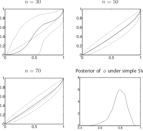
The plots of the posterior expectation ofFφ(n), together with the 95% credible interval, for each value ofnare shown in Fig-ure 1. Following referee advice we also display the estimate of the posterior density ofφ under a simple SV model for com-parison. The posterior expectation ofFφ(n)becomes closer to the true generating cumulative distribution function asnincreases; the credible interval also becomes narrower. A closer look at the plots reveals a bimodal distribution forn=30 which changes to unimodal forn=50 andn=70.These results indicate that
Fφ(n)begins to converge aroundn=50, which is not surprising since the data are generated with 50 underlining AR(1) pro-cesses. The median ofφforn=50 andn=70 appears to be within (0.7,0.8).The posterior density ofφ under the simple SV model also hints to a median within (0.7,0.8).
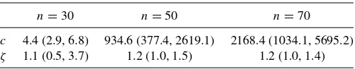
Table1displays the posterior median and 95% credible in-tervals for the concentration parameter cand ζ. The median of c increases substantially as n increases. From 4.4 ifn=
30 to 934.6 ifn=50. Given the properties of the Dirichlet
Table 1. Simulated data: the posterior median and 95% credible interval forcandζforn=30, n=50,andn=70
n=30 n=50 n=70
c 4.4 (2.9, 6.8) 934.6 (377.4, 2619.1) 2168.4 (1034.1, 5695.2) ζ 1.1 (0.5, 3.7) 1.2 (1.0, 1.5) 1.2 (1.0, 1.4)
n= 30 n= 50
0 0.5 1
0 0.2 0.4 0.6 0.8 1
0 0.5 1
0 0.2 0.4 0.6 0.8 1
n= 70 Posterior of φunder simple SV
0 0.5 1
0 0.2 0.4 0.6 0.8 1
0.4 0.6 0.8 1 0
2 4 6 8
Figure 1. Simulated data: the true cumulative distribution function (dashed line) with the posterior expectation ofFφ(n)(solid line), and 95% credible interval (dot-dashed lines) forn=30, n=50,andn=70. Thex-axis isφand they-axis is the posterior expectation ofFφ(n).The bottom right-hand graph is that of the posterior density ofφunder the simple SV model.
process, the var [Fφ(n)] becomes smaller and smaller showing thatFφ(n)is close to the centering distribution. This indicates the correct data-generating mechanism. The median ofζ changes from 1.1 to 1.2 when nincreases to 50 and settles at 1.2 even withn=70, which is consistent with our choice ofσ2.
4.2 Real Data
The real data series used to illustrate our method are: the daily returns of HSBC plc from May 16th 2000, to July 14th 2010, and the daily returns of Apple Inc. from January 1st 2000 to July 26th 2010.
Table 2. HSBC data: the posterior median and 95% credible interval forcandζforn=30, n=50,andn=70
n=30 n=50 n=70
c 5.3 (3.3, 8.4) 9.1 (6.3, 13.4) 14.3 (10.5, 19.6) ζ 1.2 (0.5, 3.8) 1.0 (0.5, 2.5) 0.9 (0.5, 1.9)
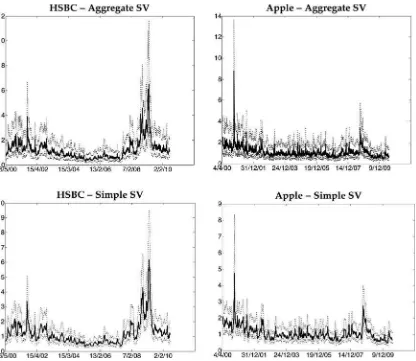
The plots of these returns are shown inFigure 2. The returns of HSBC appear more volatile than those of Apple. There is a period of relatively low volatility for HSBC from March 2003 till February 2008, with two periods of high volatility, one from October 2000 to November 2002 (the biggest dip in returns oc-curring around 9/11), and the other from January 2008 to March 2009. This latter period is due to the collapse of the banking sector following the collapse of the U.S. subprime mortgage market. In March 2009, HSBC incurred a loss of $17 billion due to its exposure to the U.S. mortgage market. The returns of Apple Inc. are not as volatile as those of HSBC plc. It operates in the technology sector where large spikes in returns are related to the effectiveness of the company in keeping up with the speed of technical advances and in launching innovative products. The period of high volatility around September 2000 is due to the introduction of the OS X operating system and the iMac which led to a 30% increase in revenue. The next high volatility period around September 2008 is due to the increase in net revenue by 50% due to the introduction of the iPhone 3G earlier in the year. As with our simulated example, we focus our attention on the convergence ofFφ(n)asnincreases. For each data series and value ofn, we provide plots of the posterior expectation ofFφ(n)
together with 95% credible intervals, as well as a plot of the estimated density ofφ under the simple SV model. We also provide the value of the posterior median (together with 95% credible intervals) ofcandζ.
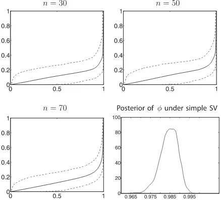
The results for HSBC are shown inFigure 3, and Tables 2
and3. The plots inFigure 3show that the posterior expectation of Fφ(n) and its 95% credible intervals are similar across the three values ofnconsidered. Focusing onn=70, we observe that much of its mass placed close to one. This is similar to the fit of a simple SV model with a single AR(1) process for
Figure 2. The returns for Apple and HSBC.
Figure 3. HSBC data: posterior expectation ofFφ(n)(solid line) with 95% credible interval (dot-dashed lines) forn=30, n=50,andn= 70.Thex-axis isφand they-axis is the posterior expectation ofFφ(n). The bottom, right-hand graph is the posterior density ofφunder the simple SV model.
ht, the volatility process. We fitted the simple SV model using the priors of Kim, Shephard, and Chib (1998) and found that
φhas a posterior median of 0.984 with a 95% credible interval (0.976, 0.992); the last plot inFigure 3confirms these findings. However, from our plots of the posterior expectation ofFφ(n)we can see that there is also mass at much smaller and much larger values ofφ.This implies that values ofφi are more spread out
within the interval (0.5,1),compared to what the simple SV model suggests.
Table2provides values for the posterior median and the 95% credible intervals for the precision parametercandζ for the three different values ofn. The median values forc, though they increase as the value ofnincreases, they are relatively small in comparison to the values we had in our simulated example. This finding means that var+Fφ(n),is large, which provides evidence to support the argument that the beta distribution (which has been the popular choice for the distribution ofφ) is not a par-ticularly good fit for the distribution ofφfor the HSBC returns, for the sample period we have analyzed.
Table 3displays the values ofγκfor various values ofκwhen
n=70. Recall thatγκis the proportion of processes with small levels of dependence less than 0.01 afterklags. The lags are displayed in terms of trading weeks and trading years.2The first
entry for γκ inTable 3indicates that 10% of the variation in volatility is explained by processes which decay after 1 week (decay quickly). Moving along the table we see that 45% of the variation is explained by processes that decay after one year. The posterior median estimate of the persistence parameter for the simple AR(1) model suggests that autocorrelation falls below 0.01 by the 286th lag. This is roughly a little over one trading year. This is an interesting point because under our model we observe that a higher proportion of the variation in volatility is
2A trading week has 5 days and a trading year approximately 252.
Figure 4. Apple data: posterior expectation ofFφ(n)(solid line) with 95% credible interval (dot-dashed lines) forn=30, n=50,andn= 70.Thex-axis isφand they-axis is the posterior expectation ofFφ(n). The bottom, right-hand graph is the posterior density ofφunder the simple SV model.
placed on processes that take 2–5 years to decay. This is clearly seen inTable 3where the autocorrelation of 19% of processes has not decayed below 0.01 after 5 years, providing evidence of very long persistence in the data.
The results for Apple are displayed in Figure 4, Tables 4, and5. The plots of the posterior expectation ofFφ(n)inFigure 4
are very similar for all three values of n. The 95% credible interval forn=30, however, is wider than those forn=50 and
n=70 (which have similar credible intervals). This implies that
Fφ(n)converges aroundn=50. Regardless of the value ofnall these plots imply thatFφ(n)for Apple is quite different to that of HSBC. With HSBC more mass was placed at higher values of
φ,whereas with Apple we see that much more mass is placed at smaller values ofφ. This difference becomes clearer when we focus on the values ofγκ, based onn=70, displayed inTable 5.
The values ofγκare larger for all lags when compared to HSBC.
In Apple’s case 85% of the variation in volatility is explained by processes with autocorrelation decaying below 0.01 before one year. In contrast, this occurs after five years (or more) with the HSBC returns series. With Apple the autocorrelation of only 4% of the processes has decayed below 0.01 after five years. This implies that the behavior of persistence in volatility is quite different between the two return series. This could be due to the two different sectors the stocks belong to and the investors belief of the riskiness not only of the two sectors but also of the two stocks.
Table 4 provides values for the posterior median and the 95% credible intervals for the precision parametercandζ for
Table 3. HSBC data: values ofγκat various lags whenn=70
1 week 2 weeks 8 weeks 1/2 year 1 year 2 years 5 years
0.10 0.16 0.26 0.38 0.45 0.54 0.81
Table 4. Apple data: the posterior median and 95% credible interval forcandζforn=30, n=50,andn=70
n=30 n=50 n=70
c 7.7 (4.6, 13.3) 445.8 (146.2, 1088.9) 3822.7 (1697.7, 9858.5) ζ 0.6 (0.3, 1.6) 0.7 (0.6,0.9) 1.0 (0.8, 1.3)
n=30, n=50,andn=70.The median value ofζmarginally increases across the three values of n, and the 95% credible intervals are narrower for the higher values ofn. The median values for c increase as the value of n increases, and in this case they are in line with the values we had in our simulated example. The median value ofcincreases to 445.8 and 3822.7 forn=50 andn=70,respectively, hinting to a small variance forFφ(n).This implies thatFφ(n) is close to a Beta distribution, unlike the results with the HSBC returns series, which hinted that the distribution forφmay not be a beta.
InFigure 5, we compare the posterior median volatility (to-gether with 95% credible interval) for HSBC and Apple under our model withn=70, to that of an SV model with a single AR(1) volatility process. The peaks and the day-to-day jumps in volatility are more evident under our model than the simple
Table 5. Apple data: the values ofγκ withn=70 for various lags
1 week 2 weeks 8 weeks 1/2 year 1 year 2 years 5 years
0.24 0.40 0.65 0.78 0.85 0.90 0.96
model. For HSBC we can identify two big jumps in volatility, one from September 2001 to November 2001 (due to 9/11) and the other from September 2008 to March 2009 (due to the start of the financial crisis following the collapse of the U.S. sub-prime mortgage market). In the case of Apple, there is one big surge in volatility around the end of September 2000 beginning of October 2000 which was due to the introduction of the OS X operating system and the iMac leading to a 30% boost of sales revenue. Since then Apple had been performing very well, with steady volatility, until September 2008 when sales revenue went up by 50% due to the introduction of the iPod touch and the iPhone 3G earlier that year.
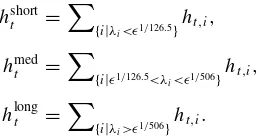
The SV-ICA model expresses the volatility process in terms of sub-processes with different levels of dependence. It is diffi-cult to interpret each individual subprocess and so we decom-pose into short-term, medium-term, and long-term components which aggregate some of these subprocesses according to their
Figure 5. Posterior median volatility for HSBC and Apple (solid line) with 95% credible interval (dashed lines) forn=70 (top panel) for the simple SV model (bottom panel).
Figure 6. The posterior mean of the high (long), medium, and low (short) frequency components of the volatility process for Apple and HSBC.
dependence. We define the components as
hshortt =
{i|λi<ǫ1/126.5}
ht,i,
hmedt =
{i|ǫ1/126.5<λ
i<ǫ1/506}
ht,i,
hlongt =
{i|λi>ǫ1/506}
ht,i.
This decomposition into components links to the quantityγκ
defined in Equation (15). The short-term component includes all processes whose dependence decays belowǫby half a year, the medium-term component includes all processes whose de-pendence decays belowǫbetween half and two years and the long-term component includes all processes whose dependence decays belowǫafter two years.
InFigure 6, we decompose the aggregate volatility process of Apple Inc. and HSBC plc, forn=70, into short-, medium-, and long-term components. The two stocks show different evo-lutions of their long-term component. The long-term component for Apple has an overall decreasing trend, whereas there is no clear overall trend for HSBC. The effect of the financial crisis also has very different effect on the volatilities with a much larger effect on HSBC compared to Apple, as we would ex-pect. The unusual observation of Apple around September and October 2000 is included in the short-term volatility compo-nent with volatility in that compocompo-nent leaping to around 2.5 and quickly decaying and with no effect on the long-term compo-nent. This shows a robustness of the SV-ICA model to unusual observations.
4.3 Predictive Performance
The predictive performance of our model is compared to a simple SV model with an AR(1) process for the log volatility and normal return distribution and a Bayesian semiparametric model proposed by Jensen and Maheu (2010). They developed a SV model with a Dirichlet process mixture model for the return distribution and an AR(1) process for the log volatility process. The comparison contrasts two ways of constructing a semiparametric SV model. Our model nonparametrically mod-els the dependence in the volatility process but retains a normal return distribution, whereas Jensen and Maheu (2010) used a nonparametric return distribution with a parametric volatility process.
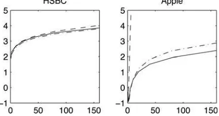
To assess predictive performance we use the log predictive score (LPS; Gneiting and Raftery2007) at different prediction horizonsτ. In this case, the LPS is
LPS(τ)= − 1
T −τ− ⌊T /2⌋ +1
T−τ
i=⌊T /2⌋
logpyiτ--y1, . . . , yi−1,
where τ is a positive integer and yiτ=yi+τ−yi is the log
return over τ days. The results are presented for time hori-zon up to 150 days. The LPS is a strictly proper scoring rule with smaller values indicating a model giving better predictions.
Figure 7displays the LPS as a function of the forecasting hori-zon. Our SV-ICA model dominates the model with a nonpara-metric return distribution at all time horizons for the Apple data and at longer time horizons for the HSBC data. In both cases, the difference becomes larger at longer time horizons. The
Figure 7. Log predictive score LPS(τ) as a function of forecasting horizon (τ). For the SV-ICA model withn=70 (solid line), the simple SV model (dot-dashed line), and the Bayesian nonparametric model (dashed line) for HSBC and Apple.
simple SV model performs well on the HSBC data (with similar predictive performance to the other models) but is outperformed by the SV-ICA model in the Apple data. These findings suggest flexible modeling of the volatility dynamics results in better predictive performance when compared to flexibly modeling the return distribution.
5. DISCUSSION
The SV-ICA model is described to flexibly model the de-pendence of the volatility process in financial time series. It is assumed that the volatility process is modeled using an ICA pro-cess which is formed as the limit of the aggregation of a finite number of AR(1) processes where the persistence parameter of each AR(1) process is independently drawn from a distribution
Fφ. The distributionFφ is a given a Bayesian nonparametric prior. The infinite-dimensional prior forFφallows our model to adjust its complexity as more data are observed. The model can be interpreted as either providing a flexible prior for persistence or, alternatively, as modeling the inhomogeneity in the infor-mation flow driving the volatility by assuming that the effect of different information decays at different rates which can be modeled by an AR(1) process. Inference is made using a finite approximation to the Dirichlet process prior forFφ withn ele-ments. Convergence can be checked by looking at the posterior distribution for various values ofn. An MCMC scheme to sim-ulate from the posterior distribution of the finite approximation is proposed which uses adaptive MCMC ideas to provide an efficient sampler.
The method is illustrated on both simulated data, where the distribution used to generate the data can be accurately esti-mated, and two daily returns series (HSBC plc and Apple Inc.). The results in the real returns series show very different distri-butions for the persistence in volatility, with HSBC plc having much more mass on persistence which decayed more slowly than Apple Inc. This suggests the information related to the value of HSBC plc has much longer lasting effect.
The decomposition of the volatility process into multiple AR(1) processes allows us to better understand the dependence in the volatility process and conclude that a flexible model for persistence is more appropriate. This is so because the volatil-ity of daily returns of stocks belonging to different sectors is affected by different flows of information. We plan in future
work to consider the application of these methods to multiple returns series which will allow us to consider the amounts of information shared by different assets. More insight on the de-pendence between return series is crucial for investment, risk, and portfolio managers.
[Received August 2012. Revised July 2013.]
REFERENCES
Arteche, J. (2004), “Gaussian Semiparametric Estimation in Long Memory in Stochastic Volatility and Signal Plus Noise Models,”Journal of Economet-rics, 119, 131–154. [102]
Atchad´e, Y. F., and Rosenthal, J. S. (2005), “On Adaptive Markov Chain Monte Carlo Algorithms,”Bernoulli, 11, 815–828. [106,107]
Bollerslev, T., and Mikkelsen, H. (1996), “Modeling and Pricing Long Memory in Stock Market Volatility,”Journal of Econometrics, 73, 151–184. [102] Breidt, F. J., Grato, N., and De Lima, P. (1998), “On the Detection and Estimation
of Long Memory in Stochastic Volatility,”Journal of Econometrics, 83, 325–348. [102]
Caron, F., and Doucet, A. (2008), “Sparse Bayesian Nonparametric Regression,” inProceedings of the 25th International Conference on Machine Learning, Helsinki, Finland. [105]
Carter, C. K., and Kohn, R. (1994), “On Gibbs Sampling for State Space Mod-els,”Biometrika, 81, 541–553. [103,106]
Cont, R. (2001), “Empirical Properties of Asset Returns: Stylized Facts and Statistical Issues,”Quantitative Finance, 1, 223–236. [102]
De Lima, P., and Grato, N. (1994), “Long-Range Dependence in the Conditional Variance of Stock Returns,”Economics Letters, 45, 281–285. [102] Ding, Z., Granger, C., and Engle, R. F. (1993), “A Long Memory Property of
Stock Market Returns and a New Model,”Journal of Empirical Finance, 1, 83–106. [102]
Ferguson, T. (1973), “Bayesian Analysis of Some Nonparametric Problems,” The Annals of Statistics, 1, 209–230. [103,104]
Fr¨uhwirth-Schnatter, S. (1994), “Data Augmentation and Dynamic Linear Mod-els,”Journal of Time Series Analysis, 15, 183–202. [103,106]
Fuller, W. (1996),Introduction to Time Series(2nd ed.), New York: Wiley. [105] Gneiting, T., and Raftery, A. E. (2007), “Strictly Proper Scoring Rules, Predic-tion and EstimaPredic-tion,”Journal of the American Statistical Association, 102, 359–378. [111]
Granger, C. (1980), “Long Memory Relationships and the Aggregation of Dy-namic Models,”Journal of Econometrics, 14, 227–238. [102,103] Griffin, J. E. (2011), “Inference in Infinite Superpositions of Non-Gaussian
Ornstein-Uhlenbeck Processes with Bayesian Nonparametric Methods,” Journal of Financial Econometrics, 9, 519–549. [103]
Griffin, J. E., and Brown, P. J. (2010), “Inference with Normal-Gamma Prior Dis-tributions in Regression Problems,”Bayesian Analysis, 5, 171–188. [105] Griffin, J. E., and Steel, M. F. J. (2004), “Semiparametric Bayesian Inference
for Stochastic Frontier Models,”Journal of Econometrics, 123, 121–152. [105]
Haario, H., Saksman, E., and Tamminen, J. (2005), “Componentwise Adap-tation for High Dimensional MCMC,” Computational Statistics, 20, 265–273. [106]
Harvey, A. (1998), “Long Memory in Stochastic Volatility,” inForecasting Volatility in Financial Markets, eds. J. Knight and S. Satchell, Oxford: Butterworth-Heineman. [102]
Hjort, N. L., Holmes, C., M¨uller, P., and Walker, S. (eds.) (2010),Bayesian Nonparametrics(1st ed.), Cambridge: Cambridge University Press. [103] Hurvich, C., Moulines, E., and Soulier, P. (2005), “Estimating Long Memory
in Volatility,”Econometrica, 73, 1283–1328. [102]
Ishwaran, H., and Zarepour, M. (2000), “Markov Chain Monte Carlo in Ap-proximate Dirichlet and Two-Parameter Process Hierarchical Models,” Biometrika, 87, 371–390. [103,105]
——— (2002), “Exact and Approximate Sum-Representations for the Dirichlet Process,” The Canadian Journal of Statistics, 30, 269– 283. [103,105]
Jensen, M. J., and Maheu, J. M. (2010), “Bayesian Semiparametric Volatility Modeling,”Journal of Econometrics, 157, 306–316. [111]
Kim, S., Shephard, N., and Chib, S. (1998), “Stochastic Volatility: Likelihood Inference and Comparison with ARCH Models,”Review of Economic Stud-ies, 65, 361–393. [103,105,109]
Latuszynski, K., Roberts, G. O., and Rosenthal, J. S. (2013), “Adaptive Gibbs Samplers and Related MCMC Methods,”The Annals of Applied Probability, 23, 66–98. [106]
Nakajima, J., and Omori, Y. (2009), “Leverage, Heavy-Tails and Correlated Jumps in Stochastic Volatility Models,”Computational Statistics & Data Analysis, 53, 2335–2353. [105]
Neal, R. (2000), “Markov Chain Sampling Methods for Dirichlet Process Mixture Models,”Journal of Computational and Graphical Statistics, 9, 249–265. [105]
Omori, Y., Chib, S., Shephard, N., and Nakajima, J. (2007), “Stochastic Volatil-ity with Leverage: Fast and Efficient Likelihood Inference,”Journal of Econometrics, 140, 28, 425–449. [105]
Richardson, S., and Green, P. (2001), “Modeling Heterogeneity with and With-out the Dirichlet Process,”Scandinavian Journal of Statistics, 355–377. [105]
Roberts, G. O., and Rosenthal, J. S. (2009), “Examples of Adaptive MCMC,” Journal of Computational and Graphical Statistics, 18, 349–367. [106]
Robinson, P. (1978), “Statistical Inference for a Randon Coefficient Autoregressive Model,” Scandinavian Journal of Statistics, 5, 163– 168. [103]
Surgailis, D., and Viano, M. (2002), “Long Memory Properties and Covariance Structure of the EGARCH Model,”ESAIM, 6, 311–329. [102]
Taylor, S. J. (1986), Modeling Financial Time Series, Chichester: Wiley. [102]
——— (2005),Asset Price Dynamics, Volatility, and PredictionPrinceton Uni-versity Press. [102]
Tsay, R. S. (2005),Analysis of Financial Time Series(2nd ed.), New York: Wiley. [102]
Zaffaroni, P. (2004), “Contemporaneous Aggregation of Linear Dynamic Models in Large Economies,” Journal of Econometrics, 120, 75– 102. [103]